Ball Mill (Perfect Mixing)

Description

This article describes an implementation of the Perfect Mixing ball mill model outlined by Napier-Munn et al. (1996).

The model described here is for steady-state simulation. For dynamic simulation, see Ball Mill (Perfect Mixing, Dynamic).

Model theory

The Perfect Mixing model is based on a population balance of particles entering the mill, breaking into smaller sizes, and discharging as product. For a mill operating in steady-state, the diagram in Figure 1 below represents the balance for a given size fraction:

Figure 1. Schematic diagram of the steady-state population balance adopted by the Perfect Mixing model.

The steady-state population balance is formulated mathematically as:

$f_{i}-R_{i}s_{i}+\sum _{j=1}^{i}{A_{ij}R_{j}s_{j}}-p_{i}=0$

where:

• $i$ is the index of the size interval, $i=\{1,2,\dots ,n\}$, $n$ is the number of size intervals
• $f_{i}$ is the mass flow rate of solids of size interval $i$ in the mill feed
• $p_{i}$ is the mass flow rate of solids of size interval $i$ in the mill product
• $s_{i}$ is the mass of solids of size interval $i$ in the mill load
• $R_{i}$ is the breakage rate of solids of size interval $i$ in the mill load
• $A_{ij}$ is the appearance function, the distribution of particle mass arising from the breakage of a parent particle in size interval $j$ into progeny of size interval $i$

As the mill is perfectly mixed, the product is related to the mill contents and discharge rate as:

$p_{i}=D_{i}s_{i}$

where $D_{i}$ is the rate of discharge of solids in size interval $i$ from the mill.

Substitution and rearrangement of the above equations leads to:

$p_{i}={\dfrac {f_{i}+\sum \limits _{j=1}^{i}{A_{ij}{\dfrac {R_{j}}{D_{j}}}p_{j}}}{1+{\dfrac {R_{i}}{D_{i}}}}}$

The mill product can therefore be computed provided a feed rate, appearance function and breakage rate per discharge rate, $R_{i}/D_{i}$, is available. Alternatively, the $R_{i}/D_{i}$ function can be determined from the feed rate, product rate and appearance function.

Discharge rate

Figure 2. Schematic of a tumbling mill showing key dimensions.

The discharge rate, $D_{i}$, is related to the residence time of pulp in the mill and can be corrected for different volumetric feed rates and mill volumes by first normalising to

$D_{i}^{*}={\dfrac {D_{i}}{\left({\dfrac {4Q_{v}}{D^{2}L}}\right)}}$

where:

• $D_{i}^{*}$ is the residence time normalised discharge rate per size interval $i$
• $Q_{v}$ is the volumetric flow rate of pulp in mill feed (solids plus liquids)
• $D$ is the mill diameter (inside liners)
• $L$ is the mill (belly) length

The actual discharge rate for a given mill and pulp feed rate is subsequently scaled as

$D_{i}=D_{i}^{*}\cdot {\dfrac {4Q_{v}}{D^{2}L}}$

with $R_{i}/D_{i}$ becoming $R_{i}/D_{i}^{*}$ for mill model calibration and simulation.

Breakage rate

The $R_{i}/D_{i}^{*}$ rate is a function of particle size and is typically a smooth, concave downward curve with a maximum related to ball size. In order to reduce the number of model parameters, the rates are specified only at three or four regularly spaced sizes (knots). Cubic spline interpolation is then used to reconstruct the complete set of rates for all size intervals.

The breakage rate, $R_{i}$, is affected by mill operating conditions and the $R_{i}/D_{i}^{*}$ rate is further scaled by the following relation:

$\left({\frac {R}{D^{*}}}\right)_{\rm {Sim}}=\left({\frac {R}{D^{*}}}\right)_{\rm {Orig}}\cdot f_{\rm {D}}\cdot f_{\rm {LF}}\cdot f_{\rm {CS}}\cdot f_{\rm {WI}}\cdot f_{\rm {Db}}$

The scaling factors are defined as:

${\begin{array}{lll}f_{\rm {D}}={\sqrt {\dfrac {D_{\rm {Sim}}}{D_{\rm {Orig}}}}},&&&f_{\rm {LF}}={\dfrac {(1-{\rm {LF}}_{\rm {Sim}}).{\rm {LF}}_{\rm {Sim}}}{(1-{\rm {LF}}_{\rm {Orig}}).{\rm {LF}}_{\rm {Orig}}}},\\f_{\rm {CS}}={\dfrac {(C_{\rm {s}})_{\rm {Sim}}}{(C_{\rm {s}})_{\rm {Orig}}}},&&&f_{\rm {WI}}=\left({\dfrac {{\rm {WI}}_{\rm {Orig}}}{{\rm {WI}}_{\rm {Sim}}}}\right)^{0.8},\\\end{array}}$

$f_{\rm {Db}}={\begin{cases}{\dfrac {Db_{\rm {Orig}}}{Db_{\rm {Sim}}}}&{\text{for }}x<x_{\rm {m(small)}},\;\;\;x_{\rm {m(small)}}=\min {\left(K.Db_{\rm {Orig}}^{2},K.Db_{\rm {Sim}}^{2}\right)}\\\left({\dfrac {Db_{\rm {Orig}}}{Db_{\rm {Sim}}}}\right)^{2}&{\text{for }}x\geq x_{\rm {m(large)}},\;\;\;x_{\rm {m(large)}}=\max {\left(K.Db_{\rm {Orig}}^{2},K.Db_{\rm {Sim}}^{2}\right)}\\\end{cases}}$

where:

• $D$ is mill diameter (m)
• ${\rm {LF}}$ is load fraction, the load volume as a fraction of mill volume (v/v)
• $C_{\rm {s}}$ is the fraction critical speed of the mill (frac)
• ${\rm {WI}}$ is the Bond Ball Work Index of the ore (kWh/t)
• $Db$ is the ball diameter (mm)
• $x$ is the diameter of a particle of size interval $i$ (mm)
• $K$ is the maximum breakage rate factor which relates ball size and the size at which $R_{i}/D_{i}^{*}$ is maximum, i.e. $x_{m}=K.Db^{2}$
• $f_{\rm {Db}}$ is interpolated for $x_{\rm {m(small)}}<x<x_{\rm {m(large)}}$

and the ${\rm {Orig}}$ subscript refers to the original mill from which $R_{i}/D_{i}^{*}$ was derived and ${\rm {Sim}}$ refers to the mill being simulated (scaled).

The grouping of breakage rate scaling factors above, excluding work index, essentially represents a relationship with mill power draw, as noted by Napier-Munn et al., King and others.

Appearance function

The appearance function describes the mass-by-size distribution of progeny particles resulting from the breakage of parent particles.

The appearance function may be specified for a particular ore. Alternatively, the default Broadbent-Callcott appearance function may be used, which is defined as:

$A_{ij}={\frac {1-\exp \left(-{\dfrac {d_{i}}{d_{j}}}\right)}{1-\exp(-1)}}$

where $d_{i}$ is the breakage product particle size and $d_{j}$ is the original particle size.

Internal mesh series

The Perfect Mixing mill model is formulated internally with a geometric progression of 31 mesh sizes at ${\sqrt {2}}$ intervals. Feed and product size fractions are automatically converted to and from the internal mesh series during model computation. The ${\sqrt {2}}$ size intervals allow the appearance function to be specified as a one-dimensional matrix, rather than the two dimensional form defined above, since

$A_{ij}=A_{i-j}$

when the intervals are so spaced.

Multi-component modelling

The original Perfect Mixing model formulation only considered the properties of a single ore type.

This implementation applies different appearance functions and breakage rate scaling factors to separate population balance computations for each ore type in the feed.

Power draw

The Perfect Mixing mill model formulation does not explicitly include a relationship with mill power draw, other than the breakage rate scaling observations noted above.

However, a simple estimate of power draw is provided for user convenience. Power is calculated according to the Morrell Empirical approach for grate and overflow discharge mills.

Excel

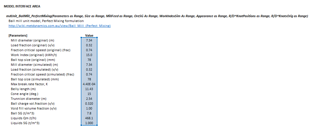
The Perfect Mixing ball mill model may be invoked from the Excel formula bar with the following function call:

=mdUnit_BallMill_PerfectMixing(Parameters as Range, Size as Range, MillFeed as Range, OreSG As Range, Appearance as Range, WorkIndexSim As Range, R/D*KnotPositions as Range, R/D*KnotsOrig as Range)

Invoking the function with no arguments will print Help text associated with the model, including a link to this page.

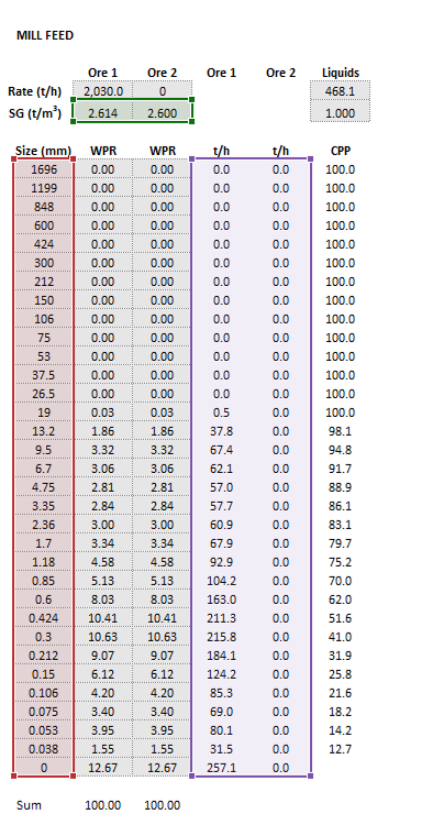
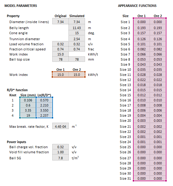
Inputs

The required inputs are defined below in matrix notation with elements corresponding to cells in Excel row ($i$) x column ($j$) format:

$Parameters={\begin{bmatrix}D_{\rm {Orig}}{\text{ (m)}}\\{\rm {LF}}_{\rm {Orig}}{\text{ (v/v)}}\\(C_{\rm {s}})_{\rm {Orig}}{\text{ (frac)}}\\{\rm {WI}}_{\rm {Orig}}{\text{ (kWh/t)}}\\Db_{\rm {Orig}}{\text{ (mm)}}\\D_{\rm {Sim}}{\text{ (m)}}\\{\rm {LF}}_{\rm {Sim}}{\text{ (v/v)}}\\(C_{\rm {s}})_{\rm {Sim}}{\text{ (frac)}}\\{\rm {WI}}_{\rm {Orig}}{\text{ (kWh/t)}}\\Db_{\rm {Sim}}{\text{ (mm)}}\\K\\L{\text{ (m)}}\\\alpha _{c}{\text{ (deg.)}}\\D_{\rm {t}}{\text{ (m)}}\\J_{\rm {B}}{\text{ (v/v)}}\\U{\text{ (v/v)}}\\\rho _{\rm {B}}{\text{ (t/m}}^{\text{3}}{\text{)}}\\(Q_{\rm {M,F}})_{\rm {L}}{\text{ (t/h)}}\\\rho _{\rm {L}}{\text{ (t/m}}^{\text{3}}{\text{)}}\\\end{bmatrix}},\;\;\;\;\;\;Size={\begin{bmatrix}d_{1}{\text{ (mm)}}\\\vdots \\d_{n}{\text{ (mm)}}\\\end{bmatrix}},\;\;\;\;\;\;MillFeed={\begin{bmatrix}(Q_{\rm {M,F}})_{11}{\text{ (t/h)}}&\dots &(Q_{\rm {M,F}})_{1m}{\text{ (t/h)}}\\\vdots &\ddots &\vdots \\(Q_{\rm {M,F}})_{n1}{\text{ (t/h)}}&\dots &(Q_{\rm {M,F}})_{nm}{\text{ (t/h)}}\\\end{bmatrix}},\;\;\;\;\;\;OreSG={\begin{bmatrix}(\rho _{\rm {S}})_{1}{\text{ (t/m}}^{\text{3}}{\text{)}}&\dots &(\rho _{\rm {S}})_{m}{\text{ (t/m}}^{\text{3}}{\text{)}}\\\end{bmatrix}}$

$Appearance={\begin{bmatrix}{\begin{bmatrix}A_{1}{\text{ (frac)}}\\\vdots \\A_{31}{\text{ (frac)}}\\\end{bmatrix}}_{1}\dots {\begin{bmatrix}A_{1}{\text{ (frac)}}\\\vdots \\A_{31}{\text{ (frac)}}\\\end{bmatrix}}_{m}\end{bmatrix}},\;\;\;\;\;\;{\rm {WI}}_{\rm {Sim}}={\begin{bmatrix}{\rm {WI}}_{1}{\text{ (kWh/t)}}&\dots &{\rm {WI}}_{m}{\text{ (kWh/t)}}\\\end{bmatrix}},\;\;\;\;\;\;R/D^{*}KnotPositions={\begin{bmatrix}d_{1}{\text{ (mm)}}\\\vdots \\d_{k}{\text{ (mm)}}\\\end{bmatrix}},\;\;\;\;\;\;R/D^{*}KnotOrig={\begin{bmatrix}\ln \left({\frac {R}{D^{*}}}\right)_{1}\\\vdots \\\ln \left({\frac {R}{D^{*}}}\right)_{k}\\\end{bmatrix}}$

where:

• $\alpha _{c}$ is angle between the cone end surface and the vertical direction (degrees)
• $D_{\rm {t}}$ is the diameter of the discharge trunnion (m)
• $J_{\rm {B}}$ is the ball charge volume fraction (typically $J_{\rm {B}}={\rm {LF}}$ for ball mills) (v/v)
• $U$ is the void fill fraction, the volumetric fraction of grinding media interstitial void space occupied by slurry (v/v)
• $\rho _{\rm {B}}$ is the Specific Gravity or density of the ball media (excluding void space) (- or t/m³)
• $(Q_{\rm {M,F}})_{\rm {L}}$ is the mass flow feed rate of liquids into the mill (t/h)
• $\rho _{\rm {L}}$ is the Specific Gravity or density of liquids in the feed (- or t/m³)
• $n$ is the number of size intervals
• $m$ is the number of ore types
• $k$ is the number of breakage rate per discharge rate knots
• $d_{i}$ is the size of the square mesh interval that feed mass is retained on (mm)
• $d_{i+1}<d_{i}<d_{i-1}$, i.e. descending size order from top size ($d_{1}$) to sub mesh ($d_{n}=0$ mm)
• $Q_{\rm {M,F}}$ is the mass flow rate of particles in the feed (t/h)
• $\rho _{\rm {S}}$ is the Specific Gravity or density of solids (- or t/m³)
• $A_{i}$ is the Appearance function value, the fraction of parent particle mass appearing in internal size interval $i$ (frac)
• ${\frac {R_{i}}{D_{i}^{*}}}$ is breakage rate per discharge rate normalised for residence time (h^-1/h^-1/h)

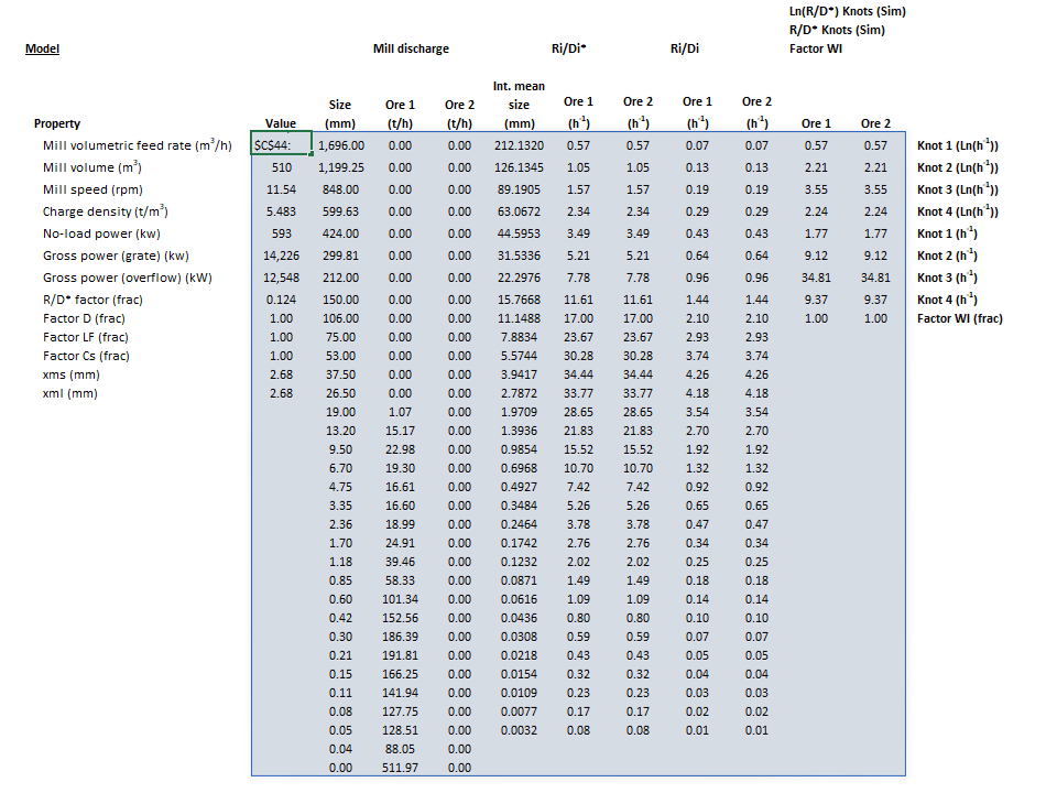
Results

The results are displayed in Excel as an array corresponding to the matrix notation below:

$mdUnit\_BallMill\_PerfectMixing={\begin{bmatrix}{\begin{bmatrix}Q_{\rm {V,F}}{\text{ (m}}^{\text{3}}{\text{/h)}}\\V{\text{ (m}}^{\text{3}}{\text{)}}\\{\text{N (rpm)}}\\\rho _{\rm {c}}{\text{ (t/m}}^{\text{3}}{\text{)}}\\{\text{No-load power (kW)}}\\{\text{Gross power (grate) (kW)}}\\{\text{Gross power (overflow) (kW)}}\\{\text{R/D* factor (-)}}\\f_{\rm {D}}{\text{ (-)}}\\f_{\rm {LF}}{\text{ (-)}}\\f_{\rm {CS}}{\text{ (-)}}\\x_{\rm {m(small)}}{\text{ (mm)}}\\x_{\rm {m(large)}}{\text{ (mm)}}\\\end{bmatrix}}&{\begin{array}{ccc}{\begin{bmatrix}d_{1}{\text{ (mm)}}\\\vdots \\d_{n}{\text{ (mm)}}\end{bmatrix}}&{\begin{bmatrix}(Q_{\rm {M,P}})_{11}{\text{ (t/h)}}&\dots &(Q_{\rm {M,P}})_{1m}{\text{ (t/h)}}\\\vdots &\ddots &\vdots \\(Q_{\rm {M,P}})_{n1}{\text{ (t/h)}}&\dots &(Q_{\rm {M,P}})_{nm}{\text{ (t/h)}}\\\end{bmatrix}}&{\begin{bmatrix}{\bar {d}}_{1}{\text{ (mm)}}\\\vdots \\{\bar {d}}_{31}{\text{ (mm)}}\\\end{bmatrix}}&{\begin{bmatrix}{\frac {R_{i}}{D_{i}^{*}}}_{11}\left({\frac {{\text{h}}^{\text{-1}}}{{\text{h}}^{\text{-1}}}}/{\text{h}}\right)&\dots &{\frac {R_{i}}{D_{i}^{*}}}_{1m}\left({\frac {{\text{h}}^{\text{-1}}}{{\text{h}}^{\text{-1}}}}/{\text{h}}\right)\\\vdots &\ddots &\vdots \\{\frac {R_{i}}{D_{i}^{*}}}_{31,1}\left({\frac {{\text{h}}^{\text{-1}}}{{\text{h}}^{\text{-1}}}}/{\text{h}}\right)&\dots &{\frac {R_{i}}{D_{i}^{*}}}_{31m}\left({\frac {{\text{h}}^{\text{-1}}}{{\text{h}}^{\text{-1}}}}/{\text{h}}\right)\\\end{bmatrix}}&{\begin{bmatrix}{\frac {R_{i}}{D_{i}}}_{11}\left({\frac {{\text{h}}^{\text{-1}}}{{\text{h}}^{\text{-1}}}}\right)&\dots &{\frac {R_{i}}{D_{i}}}_{1m}\left({\frac {{\text{h}}^{\text{-1}}}{{\text{h}}^{\text{-1}}}}\right)\\\vdots &\ddots &\vdots \\{\frac {R_{i}}{D_{i}}}_{31,1}\left({\frac {{\text{h}}^{\text{-1}}}{{\text{h}}^{\text{-1}}}}\right)&\dots &{\frac {R_{i}}{D_{i}}}_{31m}\left({\frac {{\text{h}}^{\text{-1}}}{{\text{h}}^{\text{-1}}}}\right)\\\end{bmatrix}}&{\begin{bmatrix}\ln \left({\frac {R_{i}}{D_{i}}}\right)_{11}&\dots &\ln \left({\frac {R_{i}}{D_{i}}}\right)_{1m}\\\vdots &\ddots &\vdots \\\ln \left({\frac {R_{i}}{D_{i}}}\right)_{k1}&\dots &\ln \left({\frac {R_{i}}{D_{i}}}\right)_{km}\\\end{bmatrix}}\\\\&&&&&{\begin{bmatrix}\left({\frac {R_{i}}{D_{i}}}\right)_{11}\left({\frac {{\text{h}}^{\text{-1}}}{{\text{h}}^{\text{-1}}}}\right)&\dots &\left({\frac {R_{i}}{D_{i}}}\right)_{1m}\left({\frac {{\text{h}}^{\text{-1}}}{{\text{h}}^{\text{-1}}}}\right)\\\vdots &\ddots &\vdots \\\left({\frac {R_{i}}{D_{i}}}\right)_{k1}\left({\frac {{\text{h}}^{\text{-1}}}{{\text{h}}^{\text{-1}}}}\right)&\dots &\left({\frac {R_{i}}{D_{i}}}\right)_{km}\left({\frac {{\text{h}}^{\text{-1}}}{{\text{h}}^{\text{-1}}}}\right)\\\end{bmatrix}}\\\\&&&&&{\begin{bmatrix}(f_{\rm {WI}})_{1}&\dots &(f_{\rm {WI}})_{m}\end{bmatrix}}\\&&&&&&\\&&&&&&\\\end{array}}\end{bmatrix}}$

where:

• $Q_{\rm {V,F}}$ is the flow rate of pulp into the mill (m³/h)
• $V$ is the total volume inside the mill, calculated as the sum of a cylinder and two frustums (m³)
• $N$ is the rotational rate of the mill (rpm)
• $\rho _{\rm {c}}$ is the combined density of the charge, including grinding media, coarse ore, slurry and void space (t/m³)
• ${\text{No-load power}}$ is the power input to the motor when the mill is rotating but empty (no balls, rocks or slurry) (kW)
• ${\text{Gross power (grate)}}$ is the total power input to the motor if the mill is configured with a grate discharge (kW)
• ${\text{Gross power (overflow)}}$ is the total power input to the motor if the mill is configured with an overflow discharge (kW)
• ${\text{R/D* factor}}=D_{i}^{*}/D_{i}$ is the discharge rate scaling factor
• $Q_{\rm {M,P}}$ is the mass flow rate of particles in the mill product (t/h)
• ${\bar {d}}_{i}$ is the geometric mean size of the internal mesh series interval that mass is retained on (mm)

Example

The images below show the selection of input arrays and output results in the Excel interface.

Figure 3. Example showing the selection of the Parameters (blue frame) array in Excel. Figure 4. Example showing the outline of the Results (light blue frame) array in Excel.

Figure 5. Example showing the selection of the Size (red frame), OreSG (green frame) and MillFeed (purple frame).

Figure 6. Example showing the selection of the Appearance (pink frame), R/D*KnotPositions (teal frame), R/D*KnotsOrig (blue frame), WorkIndexSim (red frame) arrays in Excel.

SysCAD

The sections and variable names used in the SysCAD interface are described in detail in the following tables.

MD_Mill page

The first tab page in the access window will have this name.

Tag (Long/Short)	Input / Display	Description/Calculated Variables/Options
Tag	Display	This name tag may be modified with the change tag option.
Condition	Display	OK if no errors/warnings, otherwise lists errors/warnings.
ConditionCount	Display	The current number of errors/warnings. If condition is OK, returns 0.
GeneralDescription / GenDesc	Display	This is an automatically generated description for the unit. If the user has entered text in the 'EqpDesc' field on the Info tab (see below), this will be displayed here. If this field is blank, then SysCAD will display the unit class ID.
Requirements
On	CheckBox	This enables the unit. If this box is not checked, then the material will pass straight through the mill with no change to the size distribution.
Method	Fixed Discharge	The discharge particle size distribution is user defined. Different distributions can be used for different solids.
	AG/SAG (Variable Rates)	The Variable Rates AG/SAG mill model is used to determine the mill product size distribution. Different parameters can be used for different solids.
	Rod Mill (Lynch)	The Lynch rod mill model is used to determine the mill product size distribution. Different parameters can be used for different solids.
	Ball (Perfect Mixing)	The Perfect Mixing ball mill model (steady-state or dynamic) is used to determine the mill product size distribution. Different parameters can be used for different solids.
	Stirred (Perfect Mixing)	The Perfect Mixing stirred mill model (steady-state or dynamic) is used to determine the mill product size distribution. Different parameters can be used for different solids.
	Mill (Herbst-Fuerstenau)	The Herbst-Fuerstenau model is used to determine the mill product size distribution. Different parameters can be used for different solids.
PowerModels	CheckBox	Show alternative mill power model calculations on the Power page.
MediaTrajectory	CheckBox	Show mill media rolling, sliding and free flight trajectory computations on the MediaTraj page.
OverfillingIndicator	CheckBox	Show overflow ball mill slurry volume, residence time, and overfilling evaluation on Overfilling page.
MediaStrings	CheckBox	Show media size distributions at recharge equilibrium on the MediaStrings page.
Options
ShowQFeed	CheckBox	QFeed and associated tab pages (eg Sp) will become visible, showing the properties of the combined feed stream.
ShowQProd	CheckBox	QProd and associated tab pages (eg Sp) will become visible, showing the properties of the products.
SizeForPassingFracCalc	Input	Size fraction for % Passing calculation. The size fraction input here will be shown in the Stream Summary section.
FracForPassingSizeCalc	Input	Fraction passing for Size calculation. The fraction input here will be shown in the Stream Summary section.
Stream Summary
MassFlow / Qm	Display	The total mass flow in each stream.
SolidMassFlow / SQm	Display	The Solids mass flow in each stream.
LiquidMassFlow / LQm	Display	The Liquid mass flow in each stream.
VolFlow / Qv	Display	The total Volume flow in each stream.
Temperature / T	Display	The Temperature of each stream.
Density / Rho	Display	The Density of each stream.
SolidFrac / Sf	Display	The Solid Fraction in each stream.
LiquidFrac / Lf	Display	The Liquid Fraction in each stream.
Passing	Display	The mass fraction passing the user-specified size (in the field SizeForPassingFracCalc) in each stream.
Passes	Display	The user-specified (in the field FracForPassesSizeCalc) fraction of material in each stream will pass this size fraction.

Mill page

The Mill page is used to specify the input parameters for the mill model.

Tag (Long/Short)	Input / Display	Description/Calculated Variables/Options
PerfectMixing
HelpLink		Opens a link to this page using the system default web browser. Note: Internet access is required.
Requirements
NumParallelUnits	Input	The number of parallel, identical units to simulate: Feed is divided by the number of parallel units before being sent to the unit model. Unit model product is multiplied back by the same value and returned to the SysCAD product stream. All unit model result values are shown per parallel unit.
MediaStringsP50	CheckBox	Only visible if the MediaStrings option is checked. Replaces the BallSize.Sim user defined value with the MediaSize (All) value from the MediaStrings page. The value of BallSize.Orig should be determined on the same basis for correct scaling of a changed media charge.
Ball
Diameter	Input	The inside liner diameter of the original and simulated ball mills.
BellyLength	Input	The inside liner belly length of the simulated ball mill, excluding cones.
ConeAngle	Input	Angle of the feed and discharge end cones, measured as positive displacement from the vertical direction.
TrunnionDiameter	Input	The inside liner trunnion diameter of the simulated ball mill.
LoadFrac	Input	The volumetric load fraction of the original and simulated ball mills.
FracCS	Input	The fraction critical speed of the original and simulated ball mills.
WorkIndex	Input	Bond Ball Work Index of ore in the original mill.
BallSize	Input	Characteristic diameter of balls in original and simulated ball mills.
MaxBreakageRateFactor / K	Input	Parameter relating ball size and the size at which the breakage rate per discharge rate is maximum.
R/DFunction
NumSplineKnots	Input	Number of spline knots for the $R_{i}/D_{i}^{*}$ function.
Size	Input	Spline knot size positions.
Ln(R/D*)	Input	Values of $\ln R/D^{*}$ at each spline knot position.
Power
BallVolume	Input	Volumetric fraction of mill occupied by balls and voids.
VoidFillFraction	Input	Volumetric fraction of void space between balls occupied by slurry.
BallSG	Input	Specific Gravity or density of ball media.
Results
MillVolume	Display	Volume inside mill, including cones.
MillSpeed	Display	Rotational speed of simulated mill.
ChargeDensity	Display	Density of charge in simulated mill, including balls, solids and liquids.
NoLoadPower	Display	Power draw of empty mill (no balls, solids or liquids)
GrossPower.Grate	Display	Gross power draw of mill in grate configuration
GrossPower.Overflow	Display	Gross power draw of mill in overflow configuration

Ore page

This page is used to define the comminution properties of SysCAD species with the size distribution quality in the project.

Tag (Long/Short)	Input / Display	Description/Calculated Variables/Options
Appearance
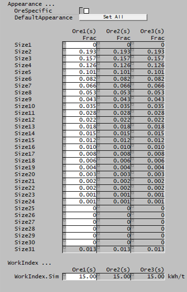
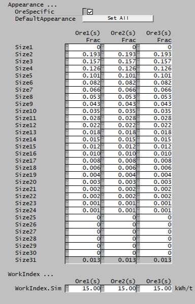
DefaultAppearance		Sets all species to the the default Broadbent-Callcott Appearance function.
OreSpecific	CheckBox	Ore-specific parameters, allows the Appearance data to be separately input for all species. Default is all species have the same set of single input properties. This option is only available if there is more than one species in the project with the size distribution property.
Appearance	Input	User-specified Appearance function data for all species with size distribution property.
WorkIndex
WorkIndex.Sim	Input	Bond Ball Work Index data for all species with size distribution property.

Ri/Di page

This page displays the scaling factors and breakage rate per discharge rate for each size interval computed by the Perfect Mixing model.

Tag (Long/Short)	Input / Display	Description/Calculated Variables/Options
Scaling
RDStar/RD	Display	Value of the ${\frac {R}{D^{*}}}{\bigg /}{\frac {R}{D}}$ factor for discharge rate scaling.
Diameter	Display	Value of the mill diameter factor for rate scaling.
LoadFraction	Display	Value of the load fraction factor for rate scaling.
FracCS	Display	Value of the fraction critical speed factor for rate scaling.
WorkIndex	Display	Value of the Work Index factor of each ore species for rate scaling.
Ri/DiStar
Size	Display	Size of each interval in internal mesh series.
MeanSize	Display	Geometric mean size of each interval in internal mesh series.
Ri/DiStar	Display	Value of normalised $R_{i}/D_{i}^{*}$ rate for each size interval, for each ore species.
Ri/Di
Size	Display	Size of each interval in internal mesh series.
MeanSize	Display	Geometric mean size of each interval in internal mesh series.
Ri/Di	Display	Value of $R_{i}/D_{i}$ rate for each size interval, for each ore species.

Power page

This optional page displays the inputs and results for alternative mill power models. The page is only visible if PowerModels is selected on the MD_Mill page.

Tag (Long/Short)	Input / Display	Description/Calculated Variables/Options
Power
HoggFuerstenau	CheckBox	Shows inputs and results for tumbling mill power calculations using the Hogg and Fuerstenau method.
MorrellC	CheckBox	Shows inputs and results for tumbling mill power calculations using the Morrell Continuum method.
MorrellE	CheckBox	Shows inputs and results for tumbling mill power calculations using the Morrell Empirical method.
MorrellD	CheckBox	Shows inputs and results for tumbling mill power calculations using the Morrell Discrete Shell method.
HildenPowell	CheckBox	Shows inputs and results for tumbling mill power calculations using the Hilden and Powell method.

MediaStrings page

This page displays the inputs and results for grinding mill media string calculations. The page is only visible if MediaStrings is selected on the MD_Mill page.

MediaTraj page

This page displays the inputs and results for tumbling mill media trajectory calculations. The page is only visible if MediaTrajectory is selected on the MD_Mill page.

Overfilling page

This page displays the inputs and results for overflow discharge mill overfilling calculations. The page is only visible if OverfillingIndicator is selected on the MD_Mill page.

About page

This page is provides product and licensing information about the Met Dynamics Models SysCAD Add-On.

Tag (Long/Short)	Input / Display	Description/Calculated Variables/Options
About
HelpLink		Opens a link to the Installation and Licensing page using the system default web browser. Note: Internet access is required.
Information		Copies Product and License information to the Windows clipboard.
Product
Name	Display	Met Dynamics software product name
Version	Display	Met Dynamics software product version number.
BuildDate	Display	Build date and time of the Met Dynamics Models SysCAD Add-On.
License
File		This is used to locate a Met Dynamics software license file.
Location	Display	Type of Met Dynamics software license or file name and path of license file.
SiteCode	Display	Unique machine identifier for license authorisation.
ReqdAuth	Display	Authorisation level required, MD-SysCAD Full or MD-SysCAD Runtime.
Status	Display	License status, LICENSE_OK indicates a valid license, other messages report licensing errors.
IssuedTo	Display	Only visible if Met Dynamics license file is used. Name of organisation/seat the license is authorised to.
ExpiryDate	Display	Only visible if Met Dynamics license file is used. License expiry date.
DaysLeft	Display	Only visible if Met Dynamics license file is used. Days left before the license expires.

See also

• Dynamic Perfect Mixing ball mill model
• Herbst-Fuerstenau mill model

References

- ↑ 1.0 1.1 Napier-Munn, T.J., Morrell, S., Morrison, R.D. and Kojovic, T., 1996. Mineral comminution circuits: their operation and optimisation. Julius Kruttschnitt Mineral Research Centre, Indooroopilly, QLD.
- ↑ King, R.P., 2012. Modeling and Simulation of Mineral Processing Systems. Elsevier.
- ↑ Gupta, A. and Yan, D.S., 2016. Mineral processing design and operations: an introduction. Elsevier.
- ↑ Morrell, S., 1996. Power draw of wet tumbling mills and its relationship to charge dynamics. Pt. 2: an empirical approach to modelling of mill power draw. Transactions of the Institution of Mining and Metallurgy. Section C. Mineral Processing and Extractive Metallurgy, 105.