Mill (Herbst-Fuerstenau): Difference between revisions
Scott Munro (talk | contribs) m (1 revision imported) |
imported>Scott.Munro m (→SysCAD) |
||
| (15 intermediate revisions by 3 users not shown) | |||
| Line 27: | Line 27: | ||
where: | where: | ||
* <math>i</math> is the index of the size interval, <math>i = \{1,2,\dots,n\}</math>, <math>n</math> is the number of size intervals | * <math>i</math> is the index of the size interval, <math>i = \{1,2,\dots,n\}</math>, <math>n</math> is the number of size intervals | ||
* <math>f_i</math> is the mass | * <math>f_i</math> is the mass fraction of particles in size interval <math>i</math> appearing in the mill feed (w/w) | ||
* <math>p_i</math> is the mass | * <math>p_i</math> is the mass fraction of particles in size interval <math>i</math> appearing in the mill product (w/w) | ||
* <math>S_i</math> is the selection function at size interval <math>i</math> | * <math>S_i</math> is the selection function at size interval <math>i</math> | ||
* <math>b_{ij}</math> is the breakage function, the mass fraction of a broken particle of original size <math>j</math> appearing in size <math>i</math> (w/w) | * <math>b_{ij}</math> is the breakage function, the mass fraction of a broken particle of original size <math>j</math> appearing in size <math>i</math> (w/w) | ||
| Line 35: | Line 35: | ||
The product of the selection function and mean residence time, <math>S_i \tau</math>, was found to be related to the energy input to grinding by: | The product of the selection function and mean residence time, <math>S_i \tau</math>, was found to be related to the energy input to grinding by: | ||
:<math>S_i \tau = S^ | :<math>S_i \tau = S^{\rm E}_i \left ( \frac{P}{W} \right ) = S^{\rm E}_i \bar E</math> | ||
where: | where: | ||
* <math>S^ | * <math>S^{\rm E}_i</math> is the ''energy-specific'' selection function at size interval <math>i</math> | ||
* <math>P</math> is the power drawn by the mill (excluding no-load power) (kW) | * <math>P</math> is the power drawn by the mill (excluding no-load power) (kW) | ||
* <math>W</math> is the mass flow rate of solids through the mill at steady-state (t/h) | * <math>W</math> is the mass flow rate of solids through the mill at steady-state (t/h) | ||
| Line 61: | Line 61: | ||
1 & i=j\\ | 1 & i=j\\ | ||
\\ | \\ | ||
\sum\limits_{k=j}^{i-1}{\dfrac{b_{ik}S^ | \sum\limits_{k=j}^{i-1}{\dfrac{b_{ik}S^{\rm E}_k}{S^{\rm E}_i - S^{\rm E}_j}}T_{kj} & i>j\\ | ||
\end{cases} | \end{cases} | ||
</math> | </math> | ||
| Line 72: | Line 72: | ||
{\rm e}^{-S_i \bar E} & \text{for batch or plug flow grinding when }i=j\\ | {\rm e}^{-S_i \bar E} & \text{for batch or plug flow grinding when }i=j\\ | ||
\\ | \\ | ||
\dfrac{1}{\left (1 + \dfrac{S^ | \dfrac{1}{\left (1 + \dfrac{S^{\rm E}_i \bar E}{N} \right )^N} & \text{for continuous grinding when }i=j\\ | ||
\\ | \\ | ||
0 & i \neq j\\ | 0 & i \neq j\\ | ||
| Line 80: | Line 80: | ||
where <math>N</math> is the number of mixers-in-series approximating the residence time distribution. | where <math>N</math> is the number of mixers-in-series approximating the residence time distribution. | ||
Different relations are available for specifying the form of the energy-specific selection (<math>S^ | Different relations are available for specifying the form of the energy-specific selection (<math>S^{\rm E}_i</math>) and breakage (<math>b_{ij}</math>) functions, which are described below. | ||
=== Energy-specific selection function === | === Energy-specific selection function === | ||
| Line 93: | Line 93: | ||
The energy-specific selection function associated with the Herbst and Fuerstenau model is:{{King (2012)}} | The energy-specific selection function associated with the Herbst and Fuerstenau model is:{{King (2012)}} | ||
:<math>S^ | :<math>S^{\rm E}_i = S^{\rm E}_1 \exp \left ( \zeta_1 \ln{ \left ( \dfrac{\bar d_{i}}{d_{{\rm p}1}} \right )} + \zeta_2 \left [ \ln{ \left ( \dfrac{\bar d_{i}}{d_{{\rm p}1}} \right )} \right ] ^2 \right )</math> | ||
where: | where: | ||
* <math>S^ | * <math>S^{\rm E}_1</math> is the value of the energy-specific selection function (<math>S^{\rm E}_i</math>) at a nominal reference particle size <math>\bar d_{{\rm p}1}</math> (mm) | ||
* <math>\bar d_{i}</math> is the [[Conversions|geometric mean size]] of particles in size interval <math>i</math> (mm) | * <math>\bar d_{i}</math> is the [[Conversions|geometric mean size]] of particles in size interval <math>i</math> (mm) | ||
* <math>\zeta_1</math> and <math>\zeta_2</math> are coefficients that characterise the shape of the energy-specific selection function curve | * <math>\zeta_1</math> and <math>\zeta_2</math> are coefficients that characterise the shape of the energy-specific selection function curve | ||
King (2012) notes the value of <math>d_{ | King (2012) notes the value of <math>d_{{\rm p}1}</math> is often taken as the top size of the mesh series in use, although a nominal size of 1mm may also be an adequate choice. | ||
==== Austin ==== | ==== Austin ==== | ||
| Line 106: | Line 106: | ||
An expanded form of the Austin selection function is available:{{Sepulveda (2005)}} | An expanded form of the Austin selection function is available:{{Sepulveda (2005)}} | ||
:<math>S^ | :<math>S^{\rm E}_i = \left( \dfrac{1}{1 + \dfrac{\alpha_2}{\alpha_1}} \right ) \left ( \dfrac{\alpha_{0} \bar {d_i}^{\alpha_{1}}}{1 + \left ( \dfrac{\bar d_i}{d_{\rm crit}} \right )^{\alpha_2}} + \alpha_{02} \bar {d_i}^{\alpha_{12}} \right )</math> | ||
where <math>\alpha_0</math>, <math>\alpha_1</math>, <math>\alpha_{2}</math>,<math>\alpha_{02}</math>, <math>\alpha_{12}</math> and <math>d_{crit}</math> are coefficients that determine the shape of the energy-specific selection function curve. | where <math>\alpha_0</math>, <math>\alpha_1</math>, <math>\alpha_{2}</math>,<math>\alpha_{02}</math>, <math>\alpha_{12}</math> and <math>d_{\rm crit}</math> are coefficients that determine the shape of the energy-specific selection function curve. | ||
The expanded function reduces to the standard Austin formulation when <math>\alpha_{02}</math> is set to zero.{{King (2012)}} | The expanded function reduces to the standard Austin formulation when <math>\alpha_{02}</math> is set to zero.{{King (2012)}} | ||
| Line 161: | Line 161: | ||
==== Natural selection ==== | ==== Natural selection ==== | ||
Vien (2019) proposed the ''natural selection function'', where the breakage function is | Vien (2019) proposed the ''natural selection function'', where the breakage function is dependent on the selection function:{{Vien (2019)}} | ||
:<math>B_{ij} = \dfrac{S^ | :<math>B_{ij} = \dfrac{S^{\rm E}_i}{S^{\rm E}_j} \implies b_{ij} = \dfrac{S^{\rm E}_{i-1} - S^{\rm E}_i}{S^{\rm E}_j}</math> | ||
The natural selection function therefore eliminates a number of parameters from the Herbst-Fuerstenau model formulation. | The natural selection function therefore eliminates a number of parameters from the Herbst-Fuerstenau model formulation. | ||
| Line 177: | Line 177: | ||
Parameters of the Herbst-Fuerstenau model may be adjusted to simulate batch laboratory mills, and continuous rod, ball and stirred mills. | Parameters of the Herbst-Fuerstenau model may be adjusted to simulate batch laboratory mills, and continuous rod, ball and stirred mills. | ||
'''Laboratory mills''' are | '''Laboratory mills''' are typically operated in batch mode. They may be simulated by applying the ''batch'' form of the population balance equations (above) and reformulating <math>\bar E</math> as: | ||
:<math>\bar E = \dfrac{P.t}{M}</math> | :<math>\bar E = \dfrac{P.t}{M}</math> | ||
| Line 215: | Line 215: | ||
MillFeed= \begin{bmatrix} | MillFeed= \begin{bmatrix} | ||
( | (Q_{\rm M,F})_{11}\text{ (t/h)} & \dots & (Q_{\rm M,F})_{1m}\text{ (t/h)}\\ | ||
\vdots & \ddots & \vdots\\ | \vdots & \ddots & \vdots\\ | ||
( | (Q_{\rm M,F})_{n1}\text{ (t/h)} & \dots & (Q_{\rm M,F})_{nm}\text{ (t/h)}\\ | ||
\end{bmatrix}</math> | \end{bmatrix}</math> | ||
{{Excel (Text, Inputs, Herbst-Fuerstenau, Selection and Breakage)}} | |||
where: | where: | ||
* <math>\text{Mixing method}</math> is the population balance equation form, ''0 = Batch/Plug Flow, 1 = Continuous'' | * <math>\text{Mixing method}</math> is the population balance equation form, ''0 = Batch/Plug Flow, 1 = Continuous'' | ||
* <math>\text{Selection method}</math> is the selection function method, 0 = User, 1 = Herbst-Fuerstenau, 2 = Austin | * <math>\text{Selection method}</math> is the selection function method, ''0 = User, 1 = Herbst-Fuerstenau, 2 = Austin'' | ||
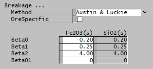
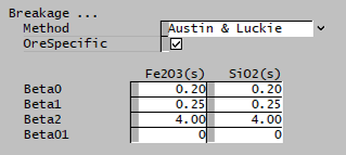
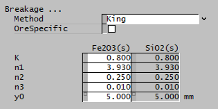
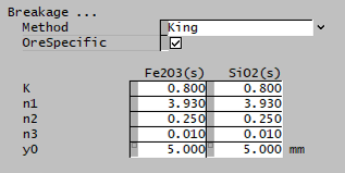
* <math>\text{Breakage method}</math> is the breakage function method, ''0 = User, 1 = Austin & Luckie, 2 = King, 3 = Natural selection'' | * <math>\text{Breakage method}</math> is the breakage function method, ''0 = User, 1 = Austin & Luckie, 2 = King, 3 = Natural selection'' | ||
* <math>m</math> is the number of ore types | * <math>m</math> is the number of ore types | ||
* <math> | * <math>Q_{\rm M,F}</math> is feed solids mass flow rate by size and ore type (t/h) | ||
=== Results === | === Results === | ||
| Line 363: | Line 241: | ||
\begin{array}{c} | \begin{array}{c} | ||
\begin{bmatrix} | |||
\bar E \text{ (kWh/t)}\\ | \bar E \text{ (kWh/t)}\\ | ||
\end{bmatrix} | |||
\\ | |||
\\ | |||
\\ | |||
\end{array} | \end{array} | ||
| Line 379: | Line 260: | ||
\begin{bmatrix} | \begin{bmatrix} | ||
( | (Q_{\rm M,P})_{11}\text{ (t/h)} & \dots & (Q_{\rm M,P})_{1m}\text{ (t/h)}\\ | ||
\vdots & \ddots & \vdots\\ | \vdots & \ddots & \vdots\\ | ||
( | (Q_{\rm M,P})_{n1}\text{ (t/h)} & \dots & (Q_{\rm M,P})_{nm}\text{ (t/h)}\\ | ||
\end{bmatrix} | \end{bmatrix} | ||
| Line 396: | Line 277: | ||
\begin{bmatrix} | \begin{bmatrix} | ||
\begin{bmatrix} | \begin{bmatrix} | ||
S^ | S^{\rm E}_1\\ | ||
\vdots\\ | \vdots\\ | ||
S^ | S^{\rm E}_n\\ | ||
\end{bmatrix}_1 | \end{bmatrix}_1 | ||
\dots | \dots | ||
\begin{bmatrix} | \begin{bmatrix} | ||
S^ | S^{\rm E}_1\\ | ||
\vdots\\ | \vdots\\ | ||
S^ | S^{\rm E}_n\\ | ||
\end{bmatrix}_m | \end{bmatrix}_m | ||
\end{bmatrix} | \end{bmatrix} | ||
| Line 427: | Line 308: | ||
</math> | </math> | ||
where <math> | where <math>Q_{\rm M,P}</math> is product mass flow rate (t/h). | ||
=== Example === | === Example === | ||
| Line 442: | Line 323: | ||
The sections and variable names used in the SysCAD interface are described in detail in the following tables. | The sections and variable names used in the SysCAD interface are described in detail in the following tables. | ||
{{SysCAD (Page, | {{SysCAD (Page, Mill, DLL*Mill)|PowerModels=true|MediaTraj=true|MediaStrings=true|Overfilling=true}} | ||
==== Mill page ==== | ==== Mill page ==== | ||
The Mill page is used to specify the input parameters for the mill model. | The Mill page is used to specify the input parameters for the mill model. | ||
{{ | {{SysCAD (Text, Table Header)}} | ||
|- | |||
! colspan="3" style="text-align:left;" |''HerbstFuerstenau'' | |||
{{SysCAD (Text, Help Link)}} | |||
|- | |- | ||
! colspan="3" style="text-align:left;" |''Requirements'' | ! colspan="3" style="text-align:left;" |''Requirements'' | ||
{{SysCAD (Text, NumParallelUnits)}} | |||
|- | |- | ||
! colspan="3" style="text-align:left;" |''Power'' | ! colspan="3" style="text-align:left;" |''Power'' | ||
|- style="vertical-align:top;" | |- style="vertical-align:top;" | ||
|rowspan=" | |rowspan="7" | Method | ||
|User | |User | ||
|The user specifies the power input to grinding. | |The user specifies the power input to grinding. | ||
|- | |- | ||
| | |HoggFuerstenau | ||
|The [[Tumbling Mill (Power, Hogg and Fuerstenau)|Hogg and Fuerstenau]] model | |The power input to grinding is the [[Tumbling Mill (Power, Hogg and Fuerstenau)|Hogg and Fuerstenau]] model ''BallsPower'' value. | ||
|- | |- | ||
|MorrellE | |MorrellE (Grate) | ||
|The [[Tumbling Mill (Power, Morrell Empirical)|Morrell Empirical]] model | |The power input to grinding is the [[Tumbling Mill (Power, Morrell Empirical)|Morrell Empirical]] model ''NetPower.Grate'' value. | ||
|- | |- | ||
|MorrellE | |MorrellE (Overflow) | ||
|The [[Tumbling Mill (Power, Morrell Empirical)|Morrell Empirical]] model | |The power input to grinding is the [[Tumbling Mill (Power, Morrell Empirical)|Morrell Empirical]] model ''NetPower.Overflow'' value. | ||
|- | |- | ||
|MorrellC | |MorrellC | ||
|The [[Tumbling Mill (Power, Morrell Continuum)|Morrell Continuum]] model | |The power input to grinding is the [[Tumbling Mill (Power, Morrell Continuum)|Morrell Continuum]] model ''NetPower'' value. | ||
|- | |- | ||
|MorrellD | |MorrellD | ||
|The [[Tumbling Mill (Power, Morrell Discrete Shell)|Morrell Discrete Shell]] model | |The power input to grinding is the [[Tumbling Mill (Power, Morrell Discrete Shell)|Morrell Discrete Shell]] model ''NetPower'' value. | ||
|- | |||
|HildenPowell | |||
|The power input to grinding is the [[Tumbling Mill (Power, Hilden and Powell)|Hilden and Powell]] model ''NetPower'' value. | |||
|- | |- | ||
|MediaPower | |MediaPower | ||
| Line 486: | Line 372: | ||
|Input | |Input | ||
|The number of mixers-in-series for grinding simulation. | |The number of mixers-in-series for grinding simulation. | ||
{{SysCAD (Text, Mill, Herbst-Fuerstenau, Selection-Breakage)}} | |||
|- | |- | ||
| Line 626: | Line 383: | ||
|} | |} | ||
{{SysCAD (Page, Mill, Herbst-Fuerstenau, Selection)}} | |||
{{ | |||
{{ | {{SysCAD (Page, Mill, Herbst-Fuerstenau, Breakage)}} | ||
{{SysCAD (Page, Tumbling Mill, Power)|modelpage={{SysCAD (Text, UnitType Prefix)}}Mill|HF=true|MorrellC=true|MorrellE=true|MorrellD=true|HildenPowell=true|Nitta=true}} | |||
| | |||
= | |||
{{ | |||
| | |||
| | |||
| | |||
| | |||
{{SysCAD (Page, Tumbling Mill, | {{SysCAD (Page, Tumbling Mill, MediaStrings)|modelpage={{SysCAD (Text, UnitType Prefix)}}Mill}} | ||
{{SysCAD (Page, Tumbling Mill, MediaTraj)|modelpage= | {{SysCAD (Page, Tumbling Mill, MediaTraj)|modelpage={{SysCAD (Text, UnitType Prefix)}}Mill}} | ||
{{SysCAD (Page, | {{SysCAD (Page, Ball Mill, Overfilling)|modelpage={{SysCAD (Text, UnitType Prefix)}}Mill}} | ||
{{SysCAD (Page, About)}} | {{SysCAD (Page, About)}} | ||
| Line 682: | Line 401: | ||
* [[Ball Mill (Perfect Mixing)|Perfect Mixing ball mill model]] | * [[Ball Mill (Perfect Mixing)|Perfect Mixing ball mill model]] | ||
* [[HPGR (Torres)|Torres HPGR model]] | * [[HPGR (Torres)|Torres HPGR model]] | ||
* [[HPGR (Campos)|Campos HPGR model]] | |||
== References == | == References == | ||
Latest revision as of 09:30, 29 May 2024
Description
This article describes an implementation of the Herbst and Fuerstenau (1980) grinding model.[1]
This model is useful for simulating batch, ball, rod and stirred mill configurations, and is a grinding power-based alternative to the (otherwise very similar) Perfect Mixing model approach.
The model is particularly flexible and offers a number of different equation options for representing the parameters of grinding.
Model theory
The Herbst-Fuerstenau model is based on a population balance of particles entering the mill, breaking into smaller sizes, and discharging as product. For a mill operating in steady-state, the diagram in Figure 1 below represents the balance for a given size fraction:
The steady-state Herbst-Fuerstenau population balance is formulated mathematically as:[2]
which may be rearranged to yield the mill product in terms of the mill feed and breakage parameters:
where:
- is the index of the size interval, , is the number of size intervals
- is the mass fraction of particles in size interval appearing in the mill feed (w/w)
- is the mass fraction of particles in size interval appearing in the mill product (w/w)
- is the selection function at size interval
- is the breakage function, the mass fraction of a broken particle of original size appearing in size (w/w)
- is the mean residence time of solids in the mill (s)
The product of the selection function and mean residence time, , was found to be related to the energy input to grinding by:
where:
- is the energy-specific selection function at size interval
- is the power drawn by the mill (excluding no-load power) (kW)
- is the mass flow rate of solids through the mill at steady-state (t/h)
- is the specific energy input to the mill (kWh/t)
The steady-state population balance model is formulated in matrix form for steady-state continuous grinding as:[1]
where:
- is a vector of the mass fractions of particles in the mill feed (w/w),
- is a vector of the mass fractions of particles in the mill product (w/w),
- and are x dimensional matrices with coefficients determined by the selection () and breakage () functions
The matrix is defined as:[3]
The matrix is different for batch, plug flow or continuous grinding"[3]
where is the number of mixers-in-series approximating the residence time distribution.
Different relations are available for specifying the form of the energy-specific selection () and breakage () functions, which are described below.
Energy-specific selection function
The following options are available for specifying the energy-specific selection function:
- Herbst and Fuerstenau
- Austin
- User defined
Herbst and Fuerstenau
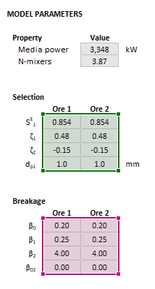
The energy-specific selection function associated with the Herbst and Fuerstenau model is:[2]
where:
- is the value of the energy-specific selection function () at a nominal reference particle size (mm)
- is the geometric mean size of particles in size interval (mm)
- and are coefficients that characterise the shape of the energy-specific selection function curve
King (2012) notes the value of is often taken as the top size of the mesh series in use, although a nominal size of 1mm may also be an adequate choice.
Austin
An expanded form of the Austin selection function is available:[4]
where , , ,, and are coefficients that determine the shape of the energy-specific selection function curve.
The expanded function reduces to the standard Austin formulation when is set to zero.[2]
User defined
The user may specify the values of the energy-specific selection function at every size interval.
This may assist in the application of additional functional forms or the analysis of experimental data.
Breakage function
The following options are available for specifying the breakage function:
- Austin and Luckie
- King
- Natural selection
- User defined
Austin and Luckie
The Austin and Luckie (1972) equation for the non-normalised cumulative breakage function is:[5][4]
where:
and:
- is the cumulative breakage function, i.e.
- , , , and are coefficients that determine the shape of the cumulative breakage function curve
The Austin and Luckie equation reduces to a normalised breakage function when is set to zero.
King
King's equation for the non-normalised cumulative breakage function is is:[2]
where , , and are coefficients that determine the shape of the cumulative breakage function curve, and is the reference parent particle size (usually assumed as 5 mm).
The King equation reduces to a normalised breakage function when is set to zero.
Natural selection
Vien (2019) proposed the natural selection function, where the breakage function is dependent on the selection function:[6]
The natural selection function therefore eliminates a number of parameters from the Herbst-Fuerstenau model formulation.
User defined
The user may specify the values of the breakage function at every parent and progeny particle size interval.
This may assist in the application of additional functional forms or the analysis of experimental data, particularly where the breakage function is non-normalisable.
Additional notes
Parameters of the Herbst-Fuerstenau model may be adjusted to simulate batch laboratory mills, and continuous rod, ball and stirred mills.
Laboratory mills are typically operated in batch mode. They may be simulated by applying the batch form of the population balance equations (above) and reformulating as:
where is the batch grinding time (s) and is the total mass of solids in the batch.
Rod mills are often assumed to operate as plug flow devices and may also be simulated by applying the batch form of the population balance equations (above).[2] No reformulation of is required in this case.
Ball mills and stirred mills are frequently assumed to be well-mixed and may be simulated by applying the continuous form of the population balance equations and specifying the number of mixers-in-series, , where appropriate.[2][7]
Excel
The Herbst-Fuerstenau mill model may be invoked from the Excel formula bar with the following function call:
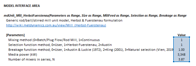
=mdUnit_Mill_HerbstFuerstenau(Parameters as Range, Size as Range, MillFeed as Range, Selection as Range, Breakage as Range)
Invoking the function with no arguments will print Help text associated with the model, including a link to this page.
Inputs
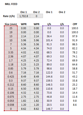
The required inputs are defined below in matrix notation with elements corresponding to cells in Excel row () x column () format:
where:
- is the population balance equation form, 0 = Batch/Plug Flow, 1 = Continuous
- is the selection function method, 0 = User, 1 = Herbst-Fuerstenau, 2 = Austin
- is the breakage function method, 0 = User, 1 = Austin & Luckie, 2 = King, 3 = Natural selection
- is the number of ore types
- is feed solids mass flow rate by size and ore type (t/h)
Results
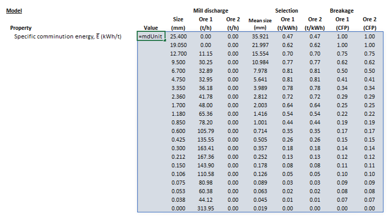
The results are displayed in Excel as an array corresponding to the matrix notation below:
where is product mass flow rate (t/h).
Example
The images below show the selection of input arrays and output results in the Excel interface.
SysCAD
The sections and variable names used in the SysCAD interface are described in detail in the following tables.
MD_Mill page
The first tab page in the access window will have this name.
| Tag (Long/Short) | Input / Display | Description/Calculated Variables/Options |
|---|---|---|
| Tag | Display | This name tag may be modified with the change tag option. |
| Condition | Display | OK if no errors/warnings, otherwise lists errors/warnings. |
| ConditionCount | Display | The current number of errors/warnings. If condition is OK, returns 0. |
| GeneralDescription / GenDesc | Display | This is an automatically generated description for the unit. If the user has entered text in the 'EqpDesc' field on the Info tab (see below), this will be displayed here.
If this field is blank, then SysCAD will display the unit class ID. |
| Requirements | ||
| On | CheckBox | This enables the unit. If this box is not checked, then the material will pass straight through the mill with no change to the size distribution. |
| Method | Fixed Discharge | The discharge particle size distribution is user defined. Different distributions can be used for different solids. |
| AG/SAG (Variable Rates) | The Variable Rates AG/SAG mill model is used to determine the mill product size distribution. Different parameters can be used for different solids. | |
| Rod Mill (Lynch) | The Lynch rod mill model is used to determine the mill product size distribution. Different parameters can be used for different solids. | |
| Ball (Perfect Mixing) | The Perfect Mixing ball mill model (steady-state or dynamic) is used to determine the mill product size distribution. Different parameters can be used for different solids. | |
| Stirred (Perfect Mixing) | The Perfect Mixing stirred mill model (steady-state or dynamic) is used to determine the mill product size distribution. Different parameters can be used for different solids. | |
| Mill (Herbst-Fuerstenau) | The Herbst-Fuerstenau model is used to determine the mill product size distribution. Different parameters can be used for different solids. | |
| PowerModels | CheckBox | Show alternative mill power model calculations on the Power page. |
| MediaTrajectory | CheckBox | Show mill media rolling, sliding and free flight trajectory computations on the MediaTraj page. |
| OverfillingIndicator | CheckBox | Show overflow ball mill slurry volume, residence time, and overfilling evaluation on Overfilling page. |
| MediaStrings | CheckBox | Show media size distributions at recharge equilibrium on the MediaStrings page. |
| Options | ||
| ShowQFeed | CheckBox | QFeed and associated tab pages (eg Sp) will become visible, showing the properties of the combined feed stream. |
| ShowQProd | CheckBox | QProd and associated tab pages (eg Sp) will become visible, showing the properties of the products. |
| SizeForPassingFracCalc | Input | Size fraction for % Passing calculation. The size fraction input here will be shown in the Stream Summary section. |
| FracForPassingSizeCalc | Input | Fraction passing for Size calculation. The fraction input here will be shown in the Stream Summary section. |
| Stream Summary | ||
| MassFlow / Qm | Display | The total mass flow in each stream. |
| SolidMassFlow / SQm | Display | The Solids mass flow in each stream. |
| LiquidMassFlow / LQm | Display | The Liquid mass flow in each stream. |
| VolFlow / Qv | Display | The total Volume flow in each stream. |
| Temperature / T | Display | The Temperature of each stream. |
| Density / Rho | Display | The Density of each stream. |
| SolidFrac / Sf | Display | The Solid Fraction in each stream. |
| LiquidFrac / Lf | Display | The Liquid Fraction in each stream. |
| Passing | Display | The mass fraction passing the user-specified size (in the field SizeForPassingFracCalc) in each stream. |
| Passes | Display | The user-specified (in the field FracForPassesSizeCalc) fraction of material in each stream will pass this size fraction. |
Mill page
The Mill page is used to specify the input parameters for the mill model.
| Tag (Long/Short) | Input / Display | Description/Calculated Variables/Options |
|---|---|---|
| HerbstFuerstenau | ||
| HelpLink | Opens a link to this page using the system default web browser. Note: Internet access is required. | |
| Requirements | ||
| NumParallelUnits | Input | The number of parallel, identical units to simulate:
|
| Power | ||
| Method | User | The user specifies the power input to grinding. |
| HoggFuerstenau | The power input to grinding is the Hogg and Fuerstenau model BallsPower value. | |
| MorrellE (Grate) | The power input to grinding is the Morrell Empirical model NetPower.Grate value. | |
| MorrellE (Overflow) | The power input to grinding is the Morrell Empirical model NetPower.Overflow value. | |
| MorrellC | The power input to grinding is the Morrell Continuum model NetPower value. | |
| MorrellD | The power input to grinding is the Morrell Discrete Shell model NetPower value. | |
| HildenPowell | The power input to grinding is the Hilden and Powell model NetPower value. | |
| MediaPower | Input/Display | Power input to grinding. The value may be user specified or linked to the selected power model on the Power page. |
| Mixing | ||
| NMixers | Input | The number of mixers-in-series for grinding simulation. |
| Selection | ||
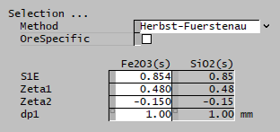
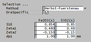
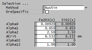
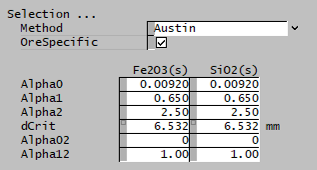
| Method | User | The user specifies the selection function. |
| Herbst and Fuerstenau | The Herbst and Fuerstenau selection function is used. | |
| Austin | The Austin selection function is used. | |
| OreSpecific | CheckBox | Ore-specific parameters, allows the selection function to be separately input for all species. Default is all species have the same set of single input properties. This option is only available if there is more than one species in the project with the size distribution property. |
| The fields below are only visible if Herbst-Fuerstenau is selected. | ||
| S1E | Input | Input parameter of the Herbst-Fuerstenau selection function. |
| Zeta1 | Input | Input parameter of the Herbst-Fuerstenau selection function. |
| Zeta2 | Input | Input parameter of the Herbst-Fuerstenau selection function. |
| dp1 | Input | Input parameter of the Herbst-Fuerstenau selection function. |
| The fields below are only visible if Austin is selected. | ||
| Alpha0 | Input | Input parameter of the Austin selection function. |
| Alpha1 | Input | Input parameter of the Austin selection function. |
| Alpha2 | Input | Input parameter of the Austin selection function. |
| dCrit | Input | Input parameter of the Austin selection function. |
| Alpha02 | Input | Input parameter of the Austin selection function. |
| Alpha12 | Input | Input parameter of the Austin selection function. |
| Breakage | ||
| Method | User | The user specifies the breakage function. |
| Austin and Luckie | The Austin and Luckie breakage function is used. | |
| King | The King selection function is used. | |
| Natural Selection | The Natural selection function is used. | |
| OreSpecific | CheckBox | Ore-specific parameters, allows the breakage function to be separately input for all species. Default is all species have the same set of single input properties. This option is only available if there is more than one species in the project with the size distribution property. |
| The fields below are only visible if Austin and Luckie is selected. | ||
| Beta0 | Input | Input parameter of the Austin and Luckie breakage function. |
| Beta1 | Input | Input parameter of the Austin and Luckie breakage function. |
| Beta2 | Input | Input parameter of the Austin and Luckie breakage function. |
| Beta01 | Input | Input parameter of the Austin and Luckie breakage function. |
| The fields below are only visible if King is selected. | ||
| K | Input | Input parameter of the King breakage function. |
| n1 | Input | Input parameter of the King breakage function. |
| n2 | Input | Input parameter of the King breakage function. |
| n3 | Input | Input parameter of the King breakage function. |
| y0 | Input | Input parameter of the King breakage function. |
| Results | ||
| Ebar | Display | Specific energy of grinding. |
Selection page
The Selection page is used to specify or display the selection function values.
| Tag (Long/Short) | Input / Display | Description/Calculated Variables/Options |
|---|---|---|
| Distribution | ||
| Name | Display | Shows the name of the SysCAD Size Distribution (PSD) quality associated with the feed stream. |
| IntervalCount | Display | Shows the number of size intervals in the SysCAD Size Distribution (PSD) quality associated with the feed stream. |
| SpWithPSDCount | Display | Shows the number of species in the feed stream assigned with the SysCAD Size Distribution (PSD) quality. |
| Selection | ||
| Size | Display | Size of each interval in mesh series. |
| MeanSize | Display | Geometric mean size of each interval in mesh series. |
| Selection | Input/Display | Value of the selection function for each size interval, for each ore species. |
Breakage page
The Breakage page is used to specify or display the breakage function values.
| Tag (Long/Short) | Input / Display | Description/Calculated Variables/Options |
|---|---|---|
| Distribution | ||
| Name | Display | Shows the name of the SysCAD Size Distribution (PSD) quality associated with the feed stream. |
| IntervalCount | Display | Shows the number of size intervals in the SysCAD Size Distribution (PSD) quality associated with the feed stream. |
| SpWithPSDCount | Display | Shows the number of species in the feed stream assigned with the SysCAD Size Distribution (PSD) quality. |
| Breakage | ||
| Size | Display | Size of each interval in internal mesh series. |
| Breakage | Input/Display | Value of the breakage function for each parent size interval, progeny size interval and ore species. |
Power page
This optional page displays the inputs and results for alternative mill power models. The page is only visible if PowerModels is selected on the MD_Mill page.
| Tag (Long/Short) | Input / Display | Description/Calculated Variables/Options |
|---|---|---|
| Power | ||
| HoggFuerstenau | CheckBox | Shows inputs and results for tumbling mill power calculations using the Hogg and Fuerstenau method. |
| MorrellC | CheckBox | Shows inputs and results for tumbling mill power calculations using the Morrell Continuum method. |
| MorrellE | CheckBox | Shows inputs and results for tumbling mill power calculations using the Morrell Empirical method. |
| MorrellD | CheckBox | Shows inputs and results for tumbling mill power calculations using the Morrell Discrete Shell method. |
| HildenPowell | CheckBox | Shows inputs and results for tumbling mill power calculations using the Hilden and Powell method. |
| Nitta | CheckBox | Shows inputs and results for stirred mill power calculations using the Nitta method. |
| Heath | CheckBox | Shows inputs and results for stirred mill power calculations using the Heath method. |
MediaStrings page
This page displays the inputs and results for grinding mill media string calculations. The page is only visible if MediaStrings is selected on the MD_Mill page.
MediaTraj page
This page displays the inputs and results for tumbling mill media trajectory calculations. The page is only visible if MediaTrajectory is selected on the MD_Mill page.
Overfilling page
This page displays the inputs and results for overflow discharge mill overfilling calculations. The page is only visible if OverfillingIndicator is selected on the MD_Mill page.
About page
This page is provides product and licensing information about the Met Dynamics Models SysCAD Add-On.
| Tag (Long/Short) | Input / Display | Description/Calculated Variables/Options |
|---|---|---|
| About | ||
| HelpLink | Opens a link to the Installation and Licensing page using the system default web browser. Note: Internet access is required. | |
| Information | Copies Product and License information to the Windows clipboard. | |
| Product | ||
| Name | Display | Met Dynamics software product name |
| Version | Display | Met Dynamics software product version number. |
| BuildDate | Display | Build date and time of the Met Dynamics Models SysCAD Add-On. |
| License | ||
| File | This is used to locate a Met Dynamics software license file. | |
| Location | Display | Type of Met Dynamics software license or file name and path of license file. |
| SiteCode | Display | Unique machine identifier for license authorisation. |
| ReqdAuth | Display | Authorisation level required, MD-SysCAD Full or MD-SysCAD Runtime. |
| Status | Display | License status, LICENSE_OK indicates a valid license, other messages report licensing errors. |
| IssuedTo | Display | Only visible if Met Dynamics license file is used. Name of organisation/seat the license is authorised to. |
| ExpiryDate | Display | Only visible if Met Dynamics license file is used. License expiry date. |
| DaysLeft | Display | Only visible if Met Dynamics license file is used. Days left before the license expires. |
See also
References
- ↑ 1.0 1.1 Herbst, J.A. and Fuerstenau, D.W., 1980. Scale-up procedure for continuous grinding mill design using population balance models. International Journal of Mineral Processing, 7(1), pp.1-31.
- ↑ 2.0 2.1 2.2 2.3 2.4 2.5 King, R.P., 2012. Modeling and Simulation of Mineral Processing Systems. Elsevier.
- ↑ 3.0 3.1 Herbst, J.A. and Rajamani, K., 1982. Developing a simulator for ball mill scale-up-a case study. Design and Installation of Comminution Circuits", Mular AL, Jergensen GV (Editors). AIME, New York, pp.325-345.
- ↑ 4.0 4.1 Sepúlveda, J., 2005. Moly-Cop Tools©. Software for the assessment and optimization of grinding-classification circuit performance.
- ↑ Austin, L.G. and Luckie, P.T., 1972. The estimation of non-normalized breakage distribution parameters from batch grinding tests. Powder Technology, 5(5), pp.267-271.
- ↑ Vien, A., 2019. The natural selection function and its application to crushing and grinding. In Proceedings of an International conference on autogenous grinding, semi-autogenous grinding and high pressure grinding roll technology.
- ↑ Mazzinghy, D.B., Schneider, C.L., Alves, V.K. and Galéry, R., 2015. Vertical agitated media mill scale-up and simulation. Minerals Engineering, 73, pp.69-76.


![{\displaystyle S_{i}^{\rm {E}}=S_{1}^{\rm {E}}\exp \left(\zeta _{1}\ln {\left({\dfrac {{\bar {d}}_{i}}{d_{{\rm {p}}1}}}\right)}+\zeta _{2}\left[\ln {\left({\dfrac {{\bar {d}}_{i}}{d_{{\rm {p}}1}}}\right)}\right]^{2}\right)}](https://wikimedia.org/api/rest_v1/media/math/render/svg/d8bb12b871366f0cd933157caac6b3a367b5d912)


![{\displaystyle Breakage={\begin{cases}{\begin{bmatrix}{\begin{bmatrix}b_{11}&&0\\\vdots &\ddots &\\b_{n1}&\dots &b_{nn}\\\end{bmatrix}}_{1}\\\vdots \\{\begin{bmatrix}b_{11}&&0\\\vdots &\ddots &\\b_{n1}&\dots &b_{nn}\\\end{bmatrix}}_{m}\\\end{bmatrix}}&{\text{ Breakage function method}}=0{\text{ (User defined)}}\\&&\\{\begin{bmatrix}{\begin{bmatrix}\beta _{0}\\\beta _{1}\\\beta _{2}\\\beta _{02}\\\end{bmatrix}}_{1}\dots {\begin{bmatrix}\beta _{0}\\\beta _{1}\\\beta _{2}\\\beta _{02}\\\end{bmatrix}}_{m}\end{bmatrix}}&{\text{ Breakage function method}}=1{\text{ (Austin and Luckie)}}\\&&\\{\begin{bmatrix}{\begin{bmatrix}K\\n_{1}\\n_{2}\\n_{3}\\y_{0}{\text{ (mm)}}\\\end{bmatrix}}_{1}\dots {\begin{bmatrix}K\\n_{1}\\n_{2}\\n_{3}\\y_{0}{\text{ (mm)}}\\\end{bmatrix}}_{m}\end{bmatrix}}&{\text{ Breakage function method}}=2{\text{ (King)}}\\&&\\{\bigg [}\;\;\;{\bigg ]}&{\text{ Breakage function method}}=3{\text{ (Natural selection)}}\\\end{cases}}}](https://wikimedia.org/api/rest_v1/media/math/render/svg/a5d17c0118ffbd4ffd94eb8f2d79ba9aa641e4ea)


