Rod Mill (Lynch): Difference between revisions
md>Scott.Munro (Created page with "== Description == This article describes an implementation of the '''Lynch''' (1977) rod mill model.{{Lynch (1977)}}{{Napier-Munn et al. (1996)}} == Model theory == {{Under...") |
imported>Scott.Munro m (→See also) |
||
| (9 intermediate revisions by 3 users not shown) | |||
| Line 4: | Line 4: | ||
== Model theory == | == Model theory == | ||
{{Restricted content}} | |||
{{ | <hide> | ||
[[File:RodMillLynch7.png|thumb|475px|Figure 1. Schematic diagram illustrating one stage of breakage (after Napier-Munn et al, 1996).{{Napier-Munn et al. (1996)}}]] | |||
Lynch (1977) describes a rod mill as a plug flow device which preferentially selects coarser particles for breakage as size reduction progresses down the mill.{{Lynch (1977)}} The preferential selection manifests as a "screening" effect which restricts the movement of coarser particles towards the discharge. | |||
To quantify this observation, Lynch defines a "stage of breakage" as the length of a mill required to completely eliminate all particles from the largest <math>\sqrt{2}</math> size interval in the feed. The product from such a stage becomes the feed for a subsequent stage, eliminating particles from the next size interval in the <math>\sqrt{2}</math> series, and so on. | |||
The size reduction in a rod mill may then be described as a series of selection, breakage and classification processes occurring in stages down the length of the mill, as illustrated schematically in Figure 1. | |||
The rod mill size reduction model was originally formulated as a sequence of matrix operations. However, this implementation adopts an equivalent algebraic population balance formulation similar to other models (e.g. [[Ball Mill (Perfect Mixing)|Perfect Mixing model]]). | |||
Thus, the product from a rod mill after <math>v</math> stages of breakage is determined from:{{Napier-Munn et al. (1996)}} | |||
:<math> | |||
\begin{align} | |||
p_{i,j} = & (1 - C_{i,j}) \cdot q_{i,j}\\ | |||
q_{i,j} = & \dfrac{(1 - S_{i,j}) \cdot p_{i,j-1} + \sum\limits_{k=1}^{i}{A_{i,k} S_{k,j} (C_{k,j} q_{k,j} + p_{k,j-1})}}{1 - C_{i,j} + S_{i,j} C_{i,j}}\\ | |||
\\ | |||
\end{align} | |||
</math> | |||
where: | |||
* <math>i</math> is the index of the size interval, <math>i = \{1,2,\dots,n\}</math>, <math>n</math> is the number of size intervals | |||
* <math>j</math> is the index of the stage of breakage, <math>j = \{1,2,\dots,v\}</math>, <math>v</math> is the number of stages of breakage, <math>v \leq n</math> | |||
* <math>f_i</math> is the mass flow rate of solids of size interval <math>i</math> in the mill feed | |||
* <math>p_{i,j}</math> is the mass flow rate of solids of size interval <math>i</math> in the product of breakage stage <math>j</math> | |||
* <math>p_{i,1} = f_i</math>, i.e. the mill feed | |||
* <math>p_{i,v}</math> is the mass flow rate of solids of size interval <math>i</math> in the product from the final stage of breakage, i.e. the mill discharge | |||
* <math>q_{i,j}</math> is the solids contents of size interval <math>i</math> in breakage stage <math>j</math> | |||
* <math>S_{i,j}</math> is the selection function, the fraction of particles of size <math>i</math> which are broken in stage <math>j</math> | |||
* <math>A_{i,k}</math> is the appearance function, the distribution of particle mass arising from the breakage of a parent particle in size interval <math>i</math> into progeny of size interval <math>k</math> | |||
* <math>C_{i,j}</math> is the classification function, the fraction of particles of size <math>i</math> in breakage stage <math>j</math> which are prevented from entering the next stage of breakage. | |||
As a model simplification, Lynch recommends the selection, appearance and classification functions are maintained constant relative to the top size of the current stage of breakage. Therefore <math>S_{i,j} = S_{i-j+1,1}</math> and <math>C_{i,j} = C_{i-j+1,1}</math> for <math>j \leq i \leq n</math>. | |||
</hide><div class="user-show"> | |||
=== Classification === | |||
</div><hide> | |||
The classification function determines the fraction of particles which are prevented from entering the next stage of breakage, i.e. that are recycled back to the feed of the current stage of breakage. | |||
The classification function adopts a simple geometric progression in order to satisfy Lynch's requirement that the top size of a breakage stage is completely eliminated. Thus, for the first stage of breakage: | |||
:<math> | |||
\begin{array}{l} | |||
C_{j=1} = | |||
\begin{bmatrix} | |||
1\\ | |||
0.5\\ | |||
0.25\\ | |||
0.125\\ | |||
0.0625\\ | |||
\vdots\\ | |||
\dfrac{1}{2(n-1)} | |||
\end{bmatrix} | |||
& | |||
\implies | |||
& | |||
C_{i,1} = | |||
\begin{cases} | |||
1 & i = 1\\ | |||
\dfrac{1}{2(i-1)} & 2 \leq i \leq n\\ | |||
\end{cases} | |||
\end{array} | |||
</math> | |||
</hide><div class="user-show"> | |||
=== Selection === | |||
</div><hide> | |||
[[File:RodMillLynch8.png|thumb|400px|Figure 2. Rod mill selection function (after Napier-Munn et al, 1996).{{Napier-Munn et al. (1996)}}]] | |||
The selection function determines the fraction of particles of a given size which are subject to breakage events. | |||
A simple linear equation is used to define the selection function, as illustrated in Figure 2. Mathematically, the selection function equation is described by: | |||
:<math> | |||
S_i = | |||
\begin{cases} | |||
{\rm SL} \cdot {\rm XC} +{\rm IN} & \bar d_i < K_1\\ | |||
{\rm SL} \cdot \bar d_i + {\rm IN} & K_1 \leq \bar d_i \leq K_2\\ | |||
1 & \bar d_i > K_2\\ | |||
\end{cases} | |||
</math> | |||
where: | |||
:<math> | |||
\begin{array}{l} | |||
K_1 = {\rm XC}, & K_2 = & \dfrac{1-{\rm IN}}{{\rm SL}}\\ | |||
\end{array} | |||
</math> | |||
and: | |||
* <math>K_1</math> and <math>K_2</math> are particle sizes with similar meanings to the same parameters used by the [[Crusher (Whiten)|Whiten crusher]] model (mm) | |||
* <math>{\rm SL}</math> is the slope of the selection function linear equation (/mm) | |||
* <math>{\rm IN}</math> is the intercept of the selection function linear equation (frac) | |||
* <math>{\rm XC}</math> is the point of intersection (mm) | |||
* <math>\bar d_{i}</math> is the [[Conversions|geometric mean size]] of particles in size interval <math>i</math> (mm) | |||
</hide><div class="user-show"> | |||
=== Appearance === | |||
</div><hide> | |||
{{Model theory (Text, Ball Mill, Perfect Mixing, Appearance)}} | |||
</hide><div class="user-show"> | |||
=== Scaling === | |||
</div><hide> | |||
</hide><div class="user-show"> | |||
==== Stages of breakage ==== | |||
</div><hide> | |||
Napier-Munn et al. (1996) suggests the number of stages of breakage of a mill to be simulated may be scaled from an original, fitted mill model by the relation:{{Napier-Munn et al. (1996)}} | |||
:<math>v_{\rm sim} = \left ( \dfrac{{\rm MC}_{\rm Sim}}{Q_{\rm M,F}} \right )^{\frac{2}{3}} + \dfrac{\ln \left ( \dfrac{(F_{90})_{\rm Orig}}{(F_{90})_{\rm Sim}} \right )}{\ln {\sqrt{2}}}</math> | |||
where: | |||
* <math>{\rm MC}</math> is the ''mill constant'', a constant that links the number of breakage stages to the mill feed rate | |||
* <math>F_{90}</math> is 90% passing size in the mill feed (mm) | |||
* <math>Q_{\rm M,F}</math> is the mass flow rate of particles in the feed (t/h) | |||
* the <math>\rm Orig</math> and <math>\rm Sim</math> subscripts refer to the original and simulated mills, respectively. | |||
The number of stages of breakage may be a non-integer value, in which case linear interpolation between stages is used to compute the mill product. | |||
</hide><div class="user-show"> | |||
==== Mill constant ==== | |||
</div><hide> | |||
The mill constant may be scaled by changes in the design or operating conditions of a mill to be simulated: | |||
:<math>{\rm MC}_{\rm Sim} = {\rm MC}_{\rm Orig} \cdot f_{\rm DL} \cdot f_{\rm LF} \cdot f_{\rm CS}</math> | |||
where: | |||
:<math> | |||
\begin{array}{l} | |||
f_{\rm DL} = \left ( \dfrac{D_{\rm Sim}}{D_{\rm Orig}} \right )^{2.5} \cdot \left ( \dfrac{L_{\rm Sim}}{L_{\rm Orig}} \right ), & | |||
f_{\rm LF} = \left ( \dfrac{1 - {\rm LF}_{\rm Sim}}{1 - {\rm LF}_{\rm Orig}} \right ) \left ( \dfrac{{\rm LF}_{\rm Sim}}{{\rm LF}_{\rm Orig}} \right ), & | |||
f_{\rm CS} = \left ( \dfrac{(\mathit{C}_{\rm s})_{\rm Sim}}{(\mathit{C}_{\rm s})_{\rm Orig}} \right )\\ | |||
\end{array} | |||
</math> | |||
and: | |||
* <math>D</math> is mill diameter (m) | |||
* <math>L</math> is mill length (m) | |||
* <math>{\rm LF}</math> is load fraction, the load volume as a fraction of mill volume (v/v) | |||
* <math>C_{\rm s}</math> is the fraction critical speed of the mill (frac) | |||
</hide><div class="user-show"> | |||
==== Ore hardness ==== | |||
</div><hide> | |||
The selection function is scaled for ore hardness by: | |||
:<math>S_{\rm Sim} = S_{\rm Orig} \cdot f_{\rm WI}</math> | |||
where: | |||
:<math>f_{\rm WI} = \left ( \dfrac{{\rm WI}_{\rm Sim}}{{\rm WI}_{\rm Orig}} \right )^{0.8}</math> | |||
and <math>{\rm WI}</math> is the Bond Rod Work Index of the ore (kWh/t). | |||
</hide><div class="user-show"> | |||
=== Internal mesh series === | |||
</div><hide> | |||
{{Model theory (Text, Ball Mill, Perfect Mixing, Internal mesh)|Lynch rod}} | |||
</hide><div class="user-show"> | |||
=== Multi-component modelling === | |||
</div><hide> | |||
The original Lynch rod mill model formulation only considered the properties of a single ore type. | |||
This implementation applies different appearance functions and selection function scaling factors to separate population balance computations for each ore type in the feed. | |||
</hide> | |||
== Excel == | == Excel == | ||
The Lynch rod mill model may be invoked from the Excel formula bar with the following function call: | The Lynch rod mill model may be invoked from the Excel formula bar with the following function call: | ||
| Line 16: | Line 191: | ||
{{Excel (Text, Help, No Arguments)}} | {{Excel (Text, Help, No Arguments)}} | ||
=== Inputs === | |||
{{Excel (Text, Inputs)}} | |||
:<math>Parameters= | |||
\begin{bmatrix} | |||
D_{\rm Orig}\text{ (m)}\\ | |||
L_{\rm Orig}\text{ (m)}\\ | |||
{\rm LF}_{\rm Orig}\text{ (v/v)}\\ | |||
(C_{\rm s})_{\rm Orig}\text{ (frac)}\\ | |||
{\rm WI}_{\rm Orig}\text{ (kWh/t)}\\ | |||
{\rm MC}_{\rm Orig}\\ | |||
(F_{90})_{\rm Orig}\text{ (mm)}\\ | |||
D_{\rm Sim}\text{ (m)}\\ | |||
L_{\rm Sim}\text{ (m)}\\ | |||
{\rm LF}_{\rm Sim}\text{ (v/v)}\\ | |||
(C_{\rm s})_{\rm Sim}\text{ (frac)}\\ | |||
\end{bmatrix},\;\;\;\;\;\; | |||
Size = \begin{bmatrix} | |||
d_{1}\text{ (mm)}\\ | |||
\vdots\\ | |||
d_n\text{ (mm)}\\ | |||
\end{bmatrix},\;\;\;\;\;\; | |||
MillFeed= \begin{bmatrix} | |||
(Q_{\rm M,F})_{11}\text{ (t/h)} & \dots & (Q_{\rm M,F})_{1m}\text{ (t/h)}\\ | |||
\vdots & \ddots & \vdots\\ | |||
(Q_{\rm M,F})_{n1}\text{ (t/h)} & \dots & (Q_{\rm M,F})_{nm}\text{ (t/h)}\\ | |||
\end{bmatrix},\;\;\;\;\;\; | |||
SelectionParams= | |||
\begin{bmatrix} | |||
{\rm XC}\text{ (mm)}\\ | |||
{\rm IN}\text{ (mm)}\\ | |||
{\rm SL}\\ | |||
\end{bmatrix} | |||
</math> | |||
:<math> | |||
Classification= | |||
\begin{bmatrix} | |||
C_{1,1}\text{ (frac)}\\ | |||
\vdots\\ | |||
C_{31,1}\text{ (frac)}\\ | |||
\end{bmatrix},\;\;\;\;\;\; | |||
Appearance= \begin{bmatrix} | |||
\begin{bmatrix} | |||
A_{1}\text{ (frac)}\\ | |||
\vdots\\ | |||
A_{31}\text{ (frac)}\\ | |||
\end{bmatrix}_1 | |||
\dots | |||
\begin{bmatrix} | |||
A_{1}\text{ (frac)}\\ | |||
\vdots\\ | |||
A_{31}\text{ (frac)}\\ | |||
\end{bmatrix}_m | |||
\end{bmatrix},\;\;\;\;\;\; | |||
{\rm WI}_{\rm Sim}= \begin{bmatrix} | |||
{\rm WI}_{1}\text{ (kWh/t)} & \dots & {\rm WI}_m\text{ (kWh/t)}\\ | |||
\end{bmatrix}\;\;\;\;\;\; | |||
</math> | |||
where: | |||
* <math>m</math> is the number of ore types | |||
* <math>d_i</math> is the size of the square mesh interval that feed mass is retained on (mm) | |||
* <math>d_{i+1}<d_i<d_{i-1}</math>, i.e. descending size order from top size (<math>d_{1}</math>) to sub mesh (<math>d_{n}=0</math> mm) | |||
=== Results === | |||
The results are displayed in Excel as an array corresponding to the matrix notation below: | |||
:<math> | |||
mdUnit\_RodlMill\_Lynch = | |||
\begin{bmatrix} | |||
\begin{bmatrix} | |||
\text{Mill speed (rpm)}\\ | |||
{\rm MC}_{\rm Sim}\\ | |||
v_{\rm Sim}\\ | |||
f_{\rm DL}\text{ (-)}\\ | |||
f_{\rm LF}\text{ (-)}\\ | |||
f_{\rm CS}\text{ (-)}\\ | |||
f_{F_{90}}\text{ (-)}\\ | |||
\end{bmatrix} | |||
& | |||
\begin{array}{cccccc} | |||
\begin{bmatrix} | |||
d_1\text{ (mm)}\\ | |||
\vdots\\ | |||
d_n\text{ (mm)} | |||
\end{bmatrix} | |||
& | |||
\begin{bmatrix} | |||
(Q_{\rm M,P})_{11}\text{ (t/h)} & \dots & (Q_{\rm M,P})_{1m}\text{ (t/h)}\\ | |||
\vdots & \ddots & \vdots\\ | |||
(Q_{\rm M,P})_{n1}\text{ (t/h)} & \dots & (Q_{\rm M,P})_{nm}\text{ (t/h)}\\ | |||
\end{bmatrix} | |||
& | |||
\begin{bmatrix} | |||
\bar{d}_1\text{ (mm)}\\ | |||
\vdots\\ | |||
\bar{d}_{31}\text{ (mm)}\\ | |||
\end{bmatrix} | |||
& | |||
\begin{bmatrix} | |||
(S_{1,1})_{\rm Orig}\text{ (frac)}\\ | |||
\vdots\\ | |||
(S_{31,1})_{\rm Orig}\text{ (frac)}\\ | |||
\end{bmatrix} | |||
& | |||
\begin{bmatrix} | |||
\begin{bmatrix} | |||
S_{1,1}\text{ (frac)}\\ | |||
\vdots\\ | |||
S_{31,1}\text{ (frac)}\\ | |||
\end{bmatrix}_1 | |||
\dots | |||
\begin{bmatrix} | |||
S_{1,1}\text{ (frac)}\\ | |||
\vdots\\ | |||
S_{31,1}\text{ (frac)}\\ | |||
\end{bmatrix}_m | |||
\end{bmatrix} | |||
& | |||
\begin{array}{c} | |||
\big [ | |||
(f_{\rm WI})_1 & \dots & (f_{\rm WI})_m | |||
\big ]\\ | |||
\\ | |||
\\ | |||
\end{array} | |||
\\ | |||
\\ | |||
\\ | |||
\\ | |||
\\ | |||
\end{array} | |||
\end{bmatrix} | |||
</math> | |||
where: | |||
* <math>\text{Mill speed}</math> is the [[Tumbling Mill (Speed)|rotational rate of the mill]] (rpm) | |||
* <math>Q_{\rm M,P}</math> is the mass flow rate of particles in the mill product (t/h) | |||
=== Example === | |||
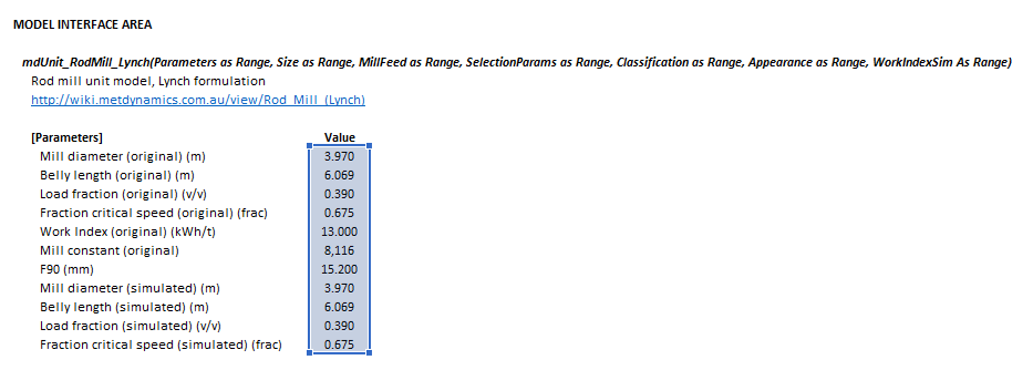
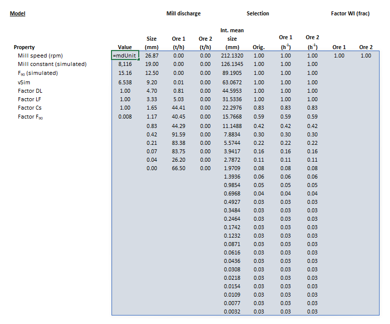
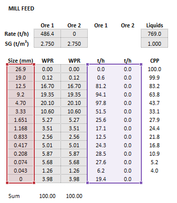
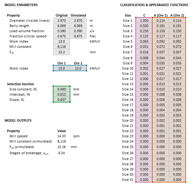
The images below show the selection of input arrays and output results in the Excel interface. | |||
{| | |||
|- style="vertical-align:top;" | |||
| [[File:RodMillLynch1.png|left|frame|Figure 1. Example showing the selection of the '''Parameters''' (blue frame) array in Excel.]] | |||
[[File:RodMillLynch4.png|left|frame|Figure 4. Example showing the outline of the '''Results''' (light blue frame) array in Excel.]] | |||
|| [[File:RodMillLynch2.png|left|frame|Figure 2. Example showing the selection of the '''Size''' (red frame) and '''MillFeed''' (purple frame).]] || [[File:RodMillLynch3.png|left|frame|Figure 3. Example showing the selection of the '''SelectionParams''' (green frame), '''Classification''' (pink frame), '''Appearance''' (brown frame), and '''WorkIndexSim''' (teal frame) arrays in Excel.]] | |||
|} | |||
== SysCAD == | == SysCAD == | ||
{{ | The sections and variable names used in the SysCAD interface are described in detail in the following tables. | ||
{{SysCAD (Page, Mill, DLL*Mill)|PowerModels=true|MediaTraj=true|MediaStrings=true}} | |||
==== Mill page ==== | |||
The Mill page is used to specify the input parameters for the mill model. | |||
{{SysCAD_Table_Header}} | |||
|- | |||
! colspan="3" style="text-align:left;" |''Lynch'' | |||
{{SysCAD (Text, Help Link)}} | |||
|- | |||
! colspan="3" style="text-align:left;" |''Scaling'' | |||
|- | |||
|Diameter | |||
|Input | |||
|The inside liner diameter of the original and simulated mills. | |||
|- | |||
|BellyLength | |||
|Input | |||
|The inside liner belly length of the simulated mill. | |||
|- | |||
|LoadFrac | |||
|Input | |||
|The volumetric load fraction of the original and simulated mills. | |||
|- | |||
|FracCS | |||
|Input | |||
|The fraction critical speed of the original and simulated mills. | |||
|- | |||
|WorkIndex | |||
|Input | |||
|Bond Rod Work Index of ore in the original mill. | |||
|- | |||
|MillConstant | |||
|Input | |||
|Mill constant of original and simulated mills. | |||
|- | |||
|F90 | |||
|Input | |||
|Size passing 90% of feed in original and simulated mills. | |||
|- | |||
! colspan="3" style="text-align:left;" |''Selection'' | |||
|- | |||
|SizeConstant / XC | |||
|Input | |||
|Size Constant value of the selection function. | |||
|- | |||
|Intercept / IN | |||
|Input | |||
|Intercept value of the selection function. | |||
|- | |||
|Slope / SL | |||
|Input | |||
|Slope value of the selection function. | |||
|- | |||
! colspan="3" style="text-align:left;" |''Results'' | |||
|- | |||
|MillSpeed | |||
|style="background: #eaecf0" | Display | |||
|Rotational speed of simulated mill. | |||
|- | |||
|NumBreakageStages | |||
|style="background: #eaecf0" | Display | |||
|Number of breakage stages in the mill. | |||
|} | |||
{{SysCAD (Page, Ball Mill, Perfect Mixing, Ore)|method=Rod}} | |||
==== Selection page ==== | |||
This page displays the selection function values computed for the Lynch rod mill model. | |||
{{SysCAD_Table_Header}} | |||
|- | |||
! colspan="3" style="text-align:left;" |''Scaling'' | |||
|- | |||
|Diameter | |||
|style="background: #eaecf0" | Display | |||
|Value of the mill diameter-length factor for rate scaling. | |||
|- | |||
|LoadFraction | |||
|style="background: #eaecf0" | Display | |||
|Value of the load fraction factor for rate scaling. | |||
|- | |||
|FracCS | |||
|style="background: #eaecf0" | Display | |||
|Value of the fraction critical speed factor for rate scaling. | |||
|- | |||
|F90 | |||
|style="background: #eaecf0" | Display | |||
|Value of the F90 factor for rate scaling. | |||
|- | |||
|WorkIndex | |||
|style="background: #eaecf0" | Display | |||
|Value of the Work Index factor of each ore species for rate scaling. | |||
|- | |||
! colspan="3" style="text-align:left;" |''Selection'' | |||
|- | |||
|Size | |||
|style="background: #eaecf0" | Display | |||
|Size of each interval in internal mesh series. | |||
|- | |||
|MeanSize | |||
|style="background: #eaecf0" | Display | |||
|Geometric mean size of each interval in internal mesh series. | |||
|- | |||
| Orig | |||
|style="background: #eaecf0" {{!}} Display | |||
| Value of original selection function at size interval. | |||
|- | |||
| Selection | |||
|style="background: #eaecf0" {{!}} Display | |||
| Value of selection function of the simulated mill for each size interval, for each ore species. | |||
|} | |||
{{SysCAD (Page, Tumbling Mill, Power)|modelpage={{SysCAD (Text, UnitType Prefix)}}Mill||HF=true|MorrellC=true|MorrellE=true}} | |||
{{SysCAD (Page, Tumbling Mill, MediaStrings)|modelpage={{SysCAD (Text, UnitType Prefix)}}Mill}} | |||
{{SysCAD (Page, Tumbling Mill, MediaTraj)|modelpage={{SysCAD (Text, UnitType Prefix)}}Mill}} | |||
{{SysCAD (Page, About)}} | |||
== See also == | |||
* [[Mill (Herbst-Fuerstenau)]] | |||
== External links == | |||
* [https://help.syscad.net/Met_Dynamics_-_Mill Met Dynamics - Mill (help.syscad.net)] | |||
== References == | == References == | ||
Latest revision as of 13:28, 1 May 2025
Description
This article describes an implementation of the Lynch (1977) rod mill model.[1][2]
Model theory
Classification
Selection
Appearance
Scaling
Stages of breakage
Mill constant
Ore hardness
Internal mesh series
Multi-component modelling
Excel
The Lynch rod mill model may be invoked from the Excel formula bar with the following function call:
=mdUnit_RodMill_Lynch(Parameters as Range, Size as Range, MillFeed as Range, SelectionParams as Range, Classification as Range, Appearance as Range, WorkIndexSim As Range)
Invoking the function with no arguments will print Help text associated with the model, including a link to this page.
Inputs
The required inputs are defined below in matrix notation with elements corresponding to cells in Excel row ([math]\displaystyle{ i }[/math]) x column ([math]\displaystyle{ j }[/math]) format:
- [math]\displaystyle{ Parameters= \begin{bmatrix} D_{\rm Orig}\text{ (m)}\\ L_{\rm Orig}\text{ (m)}\\ {\rm LF}_{\rm Orig}\text{ (v/v)}\\ (C_{\rm s})_{\rm Orig}\text{ (frac)}\\ {\rm WI}_{\rm Orig}\text{ (kWh/t)}\\ {\rm MC}_{\rm Orig}\\ (F_{90})_{\rm Orig}\text{ (mm)}\\ D_{\rm Sim}\text{ (m)}\\ L_{\rm Sim}\text{ (m)}\\ {\rm LF}_{\rm Sim}\text{ (v/v)}\\ (C_{\rm s})_{\rm Sim}\text{ (frac)}\\ \end{bmatrix},\;\;\;\;\;\; Size = \begin{bmatrix} d_{1}\text{ (mm)}\\ \vdots\\ d_n\text{ (mm)}\\ \end{bmatrix},\;\;\;\;\;\; MillFeed= \begin{bmatrix} (Q_{\rm M,F})_{11}\text{ (t/h)} & \dots & (Q_{\rm M,F})_{1m}\text{ (t/h)}\\ \vdots & \ddots & \vdots\\ (Q_{\rm M,F})_{n1}\text{ (t/h)} & \dots & (Q_{\rm M,F})_{nm}\text{ (t/h)}\\ \end{bmatrix},\;\;\;\;\;\; SelectionParams= \begin{bmatrix} {\rm XC}\text{ (mm)}\\ {\rm IN}\text{ (mm)}\\ {\rm SL}\\ \end{bmatrix} }[/math]
- [math]\displaystyle{ Classification= \begin{bmatrix} C_{1,1}\text{ (frac)}\\ \vdots\\ C_{31,1}\text{ (frac)}\\ \end{bmatrix},\;\;\;\;\;\; Appearance= \begin{bmatrix} \begin{bmatrix} A_{1}\text{ (frac)}\\ \vdots\\ A_{31}\text{ (frac)}\\ \end{bmatrix}_1 \dots \begin{bmatrix} A_{1}\text{ (frac)}\\ \vdots\\ A_{31}\text{ (frac)}\\ \end{bmatrix}_m \end{bmatrix},\;\;\;\;\;\; {\rm WI}_{\rm Sim}= \begin{bmatrix} {\rm WI}_{1}\text{ (kWh/t)} & \dots & {\rm WI}_m\text{ (kWh/t)}\\ \end{bmatrix}\;\;\;\;\;\; }[/math]
where:
- [math]\displaystyle{ m }[/math] is the number of ore types
- [math]\displaystyle{ d_i }[/math] is the size of the square mesh interval that feed mass is retained on (mm)
- [math]\displaystyle{ d_{i+1}\lt d_i\lt d_{i-1} }[/math], i.e. descending size order from top size ([math]\displaystyle{ d_{1} }[/math]) to sub mesh ([math]\displaystyle{ d_{n}=0 }[/math] mm)
Results
The results are displayed in Excel as an array corresponding to the matrix notation below:
- [math]\displaystyle{ mdUnit\_RodlMill\_Lynch = \begin{bmatrix} \begin{bmatrix} \text{Mill speed (rpm)}\\ {\rm MC}_{\rm Sim}\\ v_{\rm Sim}\\ f_{\rm DL}\text{ (-)}\\ f_{\rm LF}\text{ (-)}\\ f_{\rm CS}\text{ (-)}\\ f_{F_{90}}\text{ (-)}\\ \end{bmatrix} & \begin{array}{cccccc} \begin{bmatrix} d_1\text{ (mm)}\\ \vdots\\ d_n\text{ (mm)} \end{bmatrix} & \begin{bmatrix} (Q_{\rm M,P})_{11}\text{ (t/h)} & \dots & (Q_{\rm M,P})_{1m}\text{ (t/h)}\\ \vdots & \ddots & \vdots\\ (Q_{\rm M,P})_{n1}\text{ (t/h)} & \dots & (Q_{\rm M,P})_{nm}\text{ (t/h)}\\ \end{bmatrix} & \begin{bmatrix} \bar{d}_1\text{ (mm)}\\ \vdots\\ \bar{d}_{31}\text{ (mm)}\\ \end{bmatrix} & \begin{bmatrix} (S_{1,1})_{\rm Orig}\text{ (frac)}\\ \vdots\\ (S_{31,1})_{\rm Orig}\text{ (frac)}\\ \end{bmatrix} & \begin{bmatrix} \begin{bmatrix} S_{1,1}\text{ (frac)}\\ \vdots\\ S_{31,1}\text{ (frac)}\\ \end{bmatrix}_1 \dots \begin{bmatrix} S_{1,1}\text{ (frac)}\\ \vdots\\ S_{31,1}\text{ (frac)}\\ \end{bmatrix}_m \end{bmatrix} & \begin{array}{c} \big [ (f_{\rm WI})_1 & \dots & (f_{\rm WI})_m \big ]\\ \\ \\ \end{array} \\ \\ \\ \\ \\ \end{array} \end{bmatrix} }[/math]
where:
- [math]\displaystyle{ \text{Mill speed} }[/math] is the rotational rate of the mill (rpm)
- [math]\displaystyle{ Q_{\rm M,P} }[/math] is the mass flow rate of particles in the mill product (t/h)
Example
The images below show the selection of input arrays and output results in the Excel interface.
SysCAD
The sections and variable names used in the SysCAD interface are described in detail in the following tables.
MD_Mill page
The first tab page in the access window will have this name.
| Tag (Long/Short) | Input / Display | Description/Calculated Variables/Options |
|---|---|---|
| Tag | Display | This name tag may be modified with the change tag option. |
| Condition | Display | OK if no errors/warnings, otherwise lists errors/warnings. |
| ConditionCount | Display | The current number of errors/warnings. If condition is OK, returns 0. |
| GeneralDescription / GenDesc | Display | This is an automatically generated description for the unit. If the user has entered text in the 'EqpDesc' field on the Info tab (see below), this will be displayed here.
If this field is blank, then SysCAD will display the unit class ID. |
| Requirements | ||
| On | CheckBox | This enables the unit. If this box is not checked, then the material will pass straight through the mill with no change to the size distribution. |
| NumParallelUnits | Input | The number of parallel, identical units to simulate:
|
| Method | Fixed Discharge | The discharge particle size distribution is user defined. Different distributions can be used for different solids. |
| AG/SAG (Variable Rates) | The Variable Rates AG/SAG mill model (steady-state or dynamic) is used to determine the mill product size distribution. Different parameters can be used for different solids. | |
| Rod Mill (Lynch) | The Lynch rod mill model is used to determine the mill product size distribution. Different parameters can be used for different solids. | |
| Ball (Perfect Mixing) | The Perfect Mixing ball mill model (steady-state or dynamic) is used to determine the mill product size distribution. Different parameters can be used for different solids. | |
| Stirred (Perfect Mixing) | The Perfect Mixing stirred mill model (steady-state or dynamic) is used to determine the mill product size distribution. Different parameters can be used for different solids. | |
| Mill (Herbst-Fuerstenau) | The Herbst-Fuerstenau model is used to determine the mill product size distribution. Different parameters can be used for different solids. | |
| PowerModels | CheckBox | Show alternative mill power model calculations on the Power page. |
| MediaTrajectory | CheckBox | Show mill media rolling, sliding and free flight trajectory computations on the MediaTraj page. |
| MediaStrings | CheckBox | Show media size distributions at recharge equilibrium on the MediaStrings page. |
| Options | ||
| ShowQFeed | CheckBox | QFeed and associated tab pages (eg Sp) will become visible, showing the properties of the combined feed stream. |
| ShowQProd | CheckBox | QProd and associated tab pages (eg Sp) will become visible, showing the properties of the products. |
| SizeForPassingFracCalc | Input | Size fraction for % Passing calculation. The size fraction input here will be shown in the Stream Summary section. |
| FracForPassingSizeCalc | Input | Fraction passing for Size calculation. The fraction input here will be shown in the Stream Summary section. |
| Stream Summary | ||
| MassFlow / Qm | Display | The total mass flow in each stream. |
| SolidMassFlow / SQm | Display | The Solids mass flow in each stream. |
| LiquidMassFlow / LQm | Display | The Liquid mass flow in each stream. |
| VolFlow / Qv | Display | The total Volume flow in each stream. |
| Temperature / T | Display | The Temperature of each stream. |
| Density / Rho | Display | The Density of each stream. |
| SolidFrac / Sf | Display | The Solid Fraction in each stream. |
| LiquidFrac / Lf | Display | The Liquid Fraction in each stream. |
| Passing | Display | The mass fraction passing the user-specified size (in the field SizeForPassingFracCalc) in each stream. |
| Passes | Display | The user-specified (in the field FracForPassesSizeCalc) fraction of material in each stream will pass this size fraction. |
Mill page
The Mill page is used to specify the input parameters for the mill model.
Ore page
This page is used to define the comminution properties of SysCAD species with the size distribution quality in the project.
| Tag (Long/Short) | Input / Display | Description/Calculated Variables/Options |
|---|---|---|
| Appearance | ||
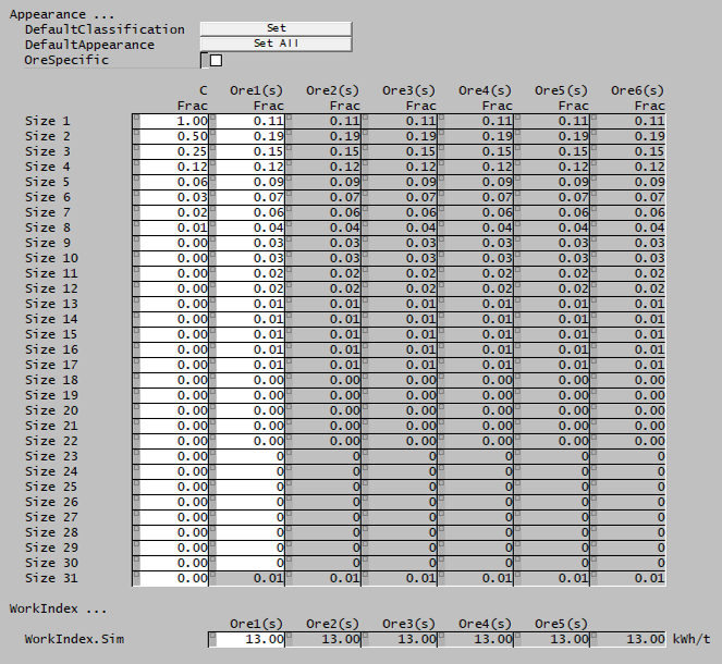
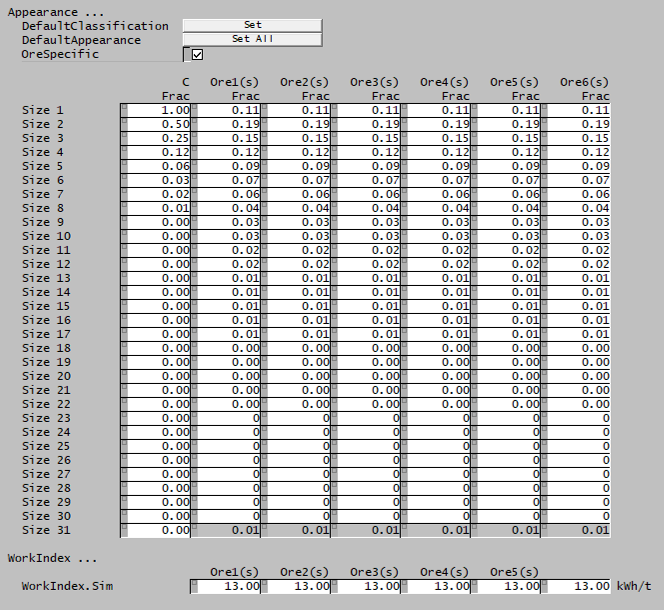
| DefaultClassification | Sets the Classification function to the default values. | |
| DefaultAppearance | Sets all species to the default Broadbent-Callcott Appearance function. | |
| OreSpecific | CheckBox |
|
| Appearance | Input | User-specified Appearance function data for all species with size distribution property. |
| WorkIndex | ||
| WorkIndex.Sim | Input | Bond Rod Work Index data for all species with size distribution property. |
Selection page
This page displays the selection function values computed for the Lynch rod mill model.
| Tag (Long/Short) | Input / Display | Description/Calculated Variables/Options |
|---|---|---|
| Scaling | ||
| Diameter | Display | Value of the mill diameter-length factor for rate scaling. |
| LoadFraction | Display | Value of the load fraction factor for rate scaling. |
| FracCS | Display | Value of the fraction critical speed factor for rate scaling. |
| F90 | Display | Value of the F90 factor for rate scaling. |
| WorkIndex | Display | Value of the Work Index factor of each ore species for rate scaling. |
| Selection | ||
| Size | Display | Size of each interval in internal mesh series. |
| MeanSize | Display | Geometric mean size of each interval in internal mesh series. |
| Orig | Display | Value of original selection function at size interval. |
| Selection | Display | Value of selection function of the simulated mill for each size interval, for each ore species. |
Power page
This optional page displays the inputs and results for alternative mill power models. The page is only visible if PowerModels is selected on the MD_Mill page.
| Tag (Long/Short) | Input / Display | Description/Calculated Variables/Options |
|---|---|---|
| Power | ||
| HoggFuerstenau | CheckBox | Shows inputs and results for tumbling mill power calculations using the Hogg and Fuerstenau method. |
| MorrellC | CheckBox | Shows inputs and results for tumbling mill power calculations using the Morrell Continuum method. |
| MorrellE | CheckBox | Shows inputs and results for tumbling mill power calculations using the Morrell Empirical method. |
MediaStrings page
This page displays the inputs and results for grinding mill media string calculations. The page is only visible if MediaStrings is selected on the MD_Mill page.
MediaTraj page
This page displays the inputs and results for tumbling mill media trajectory calculations. The page is only visible if MediaTrajectory is selected on the MD_Mill page.
About page
This page is provides product and licensing information about the Met Dynamics Models SysCAD Add-On.
| Tag (Long/Short) | Input / Display | Description/Calculated Variables/Options |
|---|---|---|
| About | ||
| HelpLink | Opens a link to the Installation and Licensing page using the system default web browser. Note: Internet access is required. | |
| Information | Copies Product and License information to the Windows clipboard. | |
| Product | ||
| Name | Display | Met Dynamics software product name |
| Version | Display | Met Dynamics software product version number. |
| BuildDate | Display | Build date and time of the Met Dynamics Models SysCAD Add-On. |
| License | ||
| File | This is used to locate a Met Dynamics software license file. | |
| Location | Display | Type of Met Dynamics software license or file name and path of license file. |
| SiteCode | Display | Unique machine identifier for license authorisation. |
| ReqdAuth | Display | Authorisation level required, MD-SysCAD Full or MD-SysCAD Runtime. |
| Status | Display | License status, LICENSE_OK indicates a valid license, other messages report licensing errors. |
| IssuedTo | Display | Only visible if Met Dynamics license file is used. Name of organisation/seat the license is authorised to. |
| ExpiryDate | Display | Only visible if Met Dynamics license file is used. License expiry date. |
| DaysLeft | Display | Only visible if Met Dynamics license file is used. Days left before the license expires. |
See also
External links
References
- ↑ Lynch, A.J., 1977. Mineral Crushing and Grinding Circuits: Their Simulation, Optimisation, Design and Control. Elsevier, Amsterdam.
- ↑ Napier-Munn, T.J., Morrell, S., Morrison, R.D. and Kojovic, T., 1996. Mineral comminution circuits: their operation and optimisation. Julius Kruttschnitt Mineral Research Centre, Indooroopilly, QLD.
