Stirred Mill (Perfect Mixing): Difference between revisions
md>Scott.Munro mNo edit summary |
imported>Scott.Munro m (→See also) |
||
| (20 intermediate revisions by 3 users not shown) | |||
| Line 1: | Line 1: | ||
== Description == | |||
This article describes an implementation of the '''Perfect Mixing''' vertical stirred mill model outlined by Napier-Munn et al. (1996).{{Napier-Munn_et_al._(1996)}} | |||
The model described here is for '''''steady-state''''' simulation. For dynamic simulation, see ''[[Stirred Mill (Perfect Mixing, Dynamic)]]''. | |||
== Model theory == | |||
{{Restricted content}} | |||
<hide> | |||
{{Model theory (Text, Mill, Perfect Mixing, Population Balance)}} | |||
</hide><div class="user-show"> | |||
=== Discharge rate === | |||
</div><hide> | |||
[[File:StirredMillDimensions1.png|thumb|425px|Figure 2. Schematic of a bottom-fed, gravity-induced vertical stirred mill showing key dimensions. The stirrer shown is a screw type with two starts and three turns per start. (After Napier-Munn et al., 1996).{{Napier-Munn et al. (1996)}}]] | |||
The discharge rate, <math>D_i</math>, is related to the residence time of pulp in the mill and can be corrected for different volumetric feed rates and mill volumes by first normalising to | |||
:<math>D_i^* = \dfrac{V_{\rm Slurry}}{Q_{\rm V}} D_i = \tau D_i</math> | |||
where: | |||
* <math>D_i^*</math> is the residence time normalised discharge rate per size interval <math>i</math> | |||
* <math>V_{\rm Slurry}</math> is the volume of slurry in the mill | |||
* <math>Q_{\rm V}</math> is the volumetric flow rate of slurry in mill feed (solids plus liquids) | |||
* <math>\tau</math> is the mean residence time of slurry in the mill | |||
The volume of slurry in the mill, <math>V_{\rm Slurry}</math> (m<sup>3</sup>), is the internal volume of the mill, <math>V_{\rm Mill}</math> (m<sup>3</sup>), minus the volume of the media, <math>V_{\rm Media}</math> (m<sup>3</sup>),: | |||
:<math>V_{\rm Slurry} = V_{\rm Mill} - V_{\rm Media} = \pi \left ( \dfrac{D}{2} \right )^2 H - \pi \left ( \dfrac{D}{2} \right )^2 H_{\rm b} (1 - \varepsilon)</math> | |||
where: | |||
* <math>D</math> is the mill diameter (m) | |||
* <math>H</math> is the mill height, the distance from the feed inlet to the product outlet (m) | |||
* <math>H_{\rm b}</math> is the height of the media charge (m) | |||
* <math>V_{\rm Stirrer}</math> is the volume occupied by the stirrer mechanism between the feed inlet to the product outlet (m<sup>3</sup>) | |||
* <math>\varepsilon</math> is volumetric fraction of interstitial void space in the charge, assumed here to be 0.4 (v/v) | |||
The volume occupied by the stirrer mechanism is ignored as a simplification. | |||
The actual discharge rate for a given mill and pulp feed rate is subsequently scaled as: | |||
:<math>D_i= \dfrac{Q_{\rm V}}{V_{\rm Slurry}} D_i^*</math> | |||
with <math>R_i/D_i</math> becoming <math>R_i/D_i^*</math> for mill model calibration and simulation. | |||
</hide><div class="user-show"> | |||
=== Breakage rate === | |||
</div><hide> | |||
The <math>R_i/D_i^*</math> rate is a function of particle size and is typically a smooth curve. In order to reduce the number of model parameters, the rates are specified only at three or four regularly spaced sizes (''knots''). Cubic spline interpolation is then used to reconstruct the complete set of rates for all size intervals. | |||
{{Model theory (Text, Stirred Mill, Perfect Mixing, Breakage Proportionality)}} | |||
Adopting the same scaling approach and nomenclature as the [[Ball Mill (Perfect Mixing)|Perfect Mixing ball mill]], the <math>R_i/D_i^*</math> rate is scaled by the following relation: | |||
:<math>\left(\frac{R}{D^*}\right)_{\rm Sim} = \left(\frac{R}{D^*}\right)_{\rm Orig} \cdot f_{\rm Ds} \cdot f_{\rm Hb} \cdot f_{\rm Ns} \cdot f_{\rm S} \cdot f_{\rm T} \cdot f_{\rm Db} \cdot f_{\rm WI}</math> | |||
{{Model theory (Text, Stirred Mill, Perfect Mixing, Breakage Scaling)}} | |||
</hide><div class="user-show"> | |||
=== Appearance function === | |||
</div><hide> | |||
{{Model theory (Text, Stirred Mill, Perfect Mixing, Appearance)}} | |||
</hide><div class="user-show"> | |||
=== Internal mesh series === | |||
</div><hide> | |||
{{Model theory (Text, Ball Mill, Perfect Mixing, Internal mesh)|Perfect Mixing}} | |||
</hide><div class="user-show"> | |||
=== Multi-component modelling === | |||
</div><hide> | |||
{{Model theory (Text, Ball Mill, Perfect Mixing, Multi-component)|Perfect Mixing|breakage rate}} | |||
</hide> | |||
== Excel == | |||
The Perfect Mixing stirred mill model may be invoked from the Excel formula bar with the following function call: | |||
<syntaxhighlight lang="vb">=mdUnit_StirredMill_PerfectMixing(Parameters as Range, Size as Range, MillFeed as Range, OreSG As Range, Appearance as Range, WorkIndexSim As Range, R/D*KnotPositions as Range, R/D*KnotsOrig as Range, Optional ScalingExponents as Range)</syntaxhighlight> | |||
{{Excel (Text, Help, No Arguments)}} | |||
=== Inputs === | |||
{{Excel (Text, Inputs)}} | |||
:<math>Parameters= | |||
\begin{bmatrix} | |||
D\text{ (m)}\\ | |||
H\text{ (m)}\\ | |||
(H_{\rm b})_{\rm Orig}\text{ (m)}\\ | |||
(D_{\rm b})_{\rm Orig}\text{ (mm)}\\ | |||
(D_{\rm s})_{\rm Orig}\text{ (m)}\\ | |||
(N_{\rm s})_{\rm Orig}\text{ (rpm)}\\ | |||
S_{\rm Orig}\\ | |||
T_{\rm Orig}\\ | |||
(H_{\rm b})_{\rm Sim}\text{ (m)}\\ | |||
(D_{\rm b})_{\rm Sim}\text{ (mm)}\\ | |||
(D_{\rm s})_{\rm Sim}\text{ (m)}\\ | |||
(N_{\rm s})_{\rm Sim}\text{ (rpm)}\\ | |||
S_{\rm Sim}\\ | |||
T_{\rm Sim}\\ | |||
{\rm WI}_{\rm Orig}\text{ (kWh/t)}\\ | |||
(Q_{\rm M,F})_{\rm L}\text{ (t/h)}\\ | |||
\rho_{\rm L}\text{ (t/m}^{\text{3}}\text{)}\\ | |||
\end{bmatrix},\;\;\;\;\;\; | |||
Size = \begin{bmatrix} | |||
d_{1}\text{ (mm)}\\ | |||
\vdots\\ | |||
d_n\text{ (mm)}\\ | |||
\end{bmatrix},\;\;\;\;\;\; | |||
MillFeed= \begin{bmatrix} | |||
(Q_{\rm M,F})_{11}\text{ (t/h)} & \dots & (Q_{\rm M,F})_{1m}\text{ (t/h)}\\ | |||
\vdots & \ddots & \vdots\\ | |||
(Q_{\rm M,F})_{n1}\text{ (t/h)} & \dots & (Q_{\rm M,F})_{nm}\text{ (t/h)}\\ | |||
\end{bmatrix},\;\;\;\;\;\; | |||
OreSG= \begin{bmatrix} | |||
(\rho_{\rm S})_{1}\text{ (t/m}^\text{3}\text{)} & \dots & (\rho_{\rm S})_m\text{ (t/m}^\text{3}\text{)}\\ | |||
\end{bmatrix} | |||
</math> | |||
:<math> | |||
Appearance= \begin{bmatrix} | |||
\begin{bmatrix} | |||
A_{1}\text{ (frac)}\\ | |||
\vdots\\ | |||
A_{31}\text{ (frac)}\\ | |||
\end{bmatrix}_1 | |||
\dots | |||
\begin{bmatrix} | |||
A_{1}\text{ (frac)}\\ | |||
\vdots\\ | |||
A_{31}\text{ (frac)}\\ | |||
\end{bmatrix}_m | |||
\end{bmatrix},\;\;\;\;\;\; | |||
{\rm WI}_{\rm Sim}= \begin{bmatrix} | |||
{\rm WI}_{1}\text{ (kWh/t)} & \dots & {\rm WI}_m\text{ (kWh/t)}\\ | |||
\end{bmatrix},\;\;\;\;\;\; | |||
R/D^*KnotPositions= \begin{bmatrix} | |||
d_{1}\text{ (mm)}\\ | |||
\vdots\\ | |||
d_{k}\text{ (mm)}\\ | |||
\end{bmatrix},\;\;\;\;\;\; | |||
R/D^*KnotOrig= \begin{bmatrix} | |||
\ln\left(\frac{R}{D^*}\right)_1\\ | |||
\vdots\\ | |||
\ln\left(\frac{R}{D^*}\right)_k\\ | |||
\end{bmatrix} | |||
</math> | |||
:<math> | |||
\mathit{ScalingExponents} = \begin{bmatrix} | |||
e_1\\ | |||
e_2\\ | |||
e_3\\ | |||
e_4\\ | |||
e_5\\ | |||
e_6\\ | |||
e_7\\ | |||
\end{bmatrix}^* | |||
</math> | |||
where: | |||
* <math>(Q_{\rm M,F})_{\rm L}</math> is the mass flow feed rate of liquids into the mill (t/h) | |||
* <math>\rho_{\rm B}</math> is the Specific Gravity or density of the media in the mill (- or t/m<sup>3</sup>) | |||
* <math>\rho_{\rm L}</math> is the Specific Gravity or density of liquids in the feed (- or t/m<sup>3</sup>) | |||
* <math>m</math> is the number of ore types | |||
* <math>k</math> is the number of breakage rate per discharge rate knots | |||
* <math>d_i</math> is the size of the square mesh interval that feed mass is retained on (mm) | |||
* <math>d_{i+1}<d_i<d_{i-1}</math>, i.e. descending size order from top size (<math>d_{1}</math>) to sub mesh (<math>d_{n}=0</math> mm) | |||
* <math>Q_{\rm M,F}</math> is the mass flow rate of particles in the feed (t/h) | |||
* <math>\rho_{\rm S}</math> is the Specific Gravity or density of solids (- or t/m<sup>3</sup>) | |||
* <math>^*</math> indicates the <math>\mathit{ScalingExponents}</math> array is optional, the default values are used if omitted. | |||
<!-- | |||
\quad \text{ or } \quad | |||
\begin{bmatrix} | |||
\ln\left(\frac{R}{D^*}\right)_{11} & \dots & \ln\left(\frac{R}{D^*}\right)_{1m}\\ | |||
\vdots & \ddots & \vdots\\ | |||
\ln\left(\frac{R}{D^*}\right)_{k1} & \dots & \ln\left(\frac{R}{D^*}\right)_{km}\\ | |||
\end{bmatrix} | |||
--> | |||
=== Results === | |||
The results are displayed in Excel as an array corresponding to the matrix notation below: | |||
:<math> | |||
mdUnit\_StirredMill\_PerfectMixing = | |||
\begin{bmatrix} | |||
\begin{bmatrix} | |||
Q_{\rm V}\text{ (m}^{\text{3}}\text{/h)}\\ | |||
V_{\rm Mill}\text{ (m}^{\text{3}}\text{)}\\ | |||
V_{\rm Media}\\ | |||
V_{\rm Slurry}\\ | |||
{\rm LF}\text{ (v/v)}\\ | |||
\tau\text{ (min)}\\ | |||
\text{R/D* factor (frac)}\\ | |||
f_{\rm Ds}\text{ (-)}\\ | |||
f_{\rm Hb}\text{ (-)}\\ | |||
f_{\rm Ns}\text{ (-)}\\ | |||
f_{\rm S}\text{ (-)}\\ | |||
f_{\rm T}\text{ (-)}\\ | |||
f_{\rm Db}\text{ (-)}\\ | |||
f_{\rm WI}\text{ (-)}\\ | |||
\end{bmatrix} | |||
& | |||
\begin{array}{cccccc} | |||
\begin{bmatrix} | |||
d_1\text{ (mm)}\\ | |||
\vdots\\ | |||
d_n\text{ (mm)} | |||
\end{bmatrix} | |||
& | |||
\begin{bmatrix} | |||
(Q_{\rm M,P})_{11}\text{ (t/h)} & \dots & (Q_{\rm M,P})_{1m}\text{ (t/h)}\\ | |||
\vdots & \ddots & \vdots\\ | |||
(Q_{\rm M,P})_{n1}\text{ (t/h)} & \dots & (Q_{\rm M,P})_{nm}\text{ (t/h)}\\ | |||
\end{bmatrix} | |||
& | |||
\begin{bmatrix} | |||
\bar{d}_1\text{ (mm)}\\ | |||
\vdots\\ | |||
\bar{d}_{31}\text{ (mm)}\\ | |||
\end{bmatrix} | |||
& | |||
\begin{bmatrix} | |||
\frac{R_i}{D_i^*}_{11}\left(\frac{\text{h}^\text{-1}}{\text{h}^\text{-1}}/\text{h}\right) & \dots & \frac{R_i}{D_i^*}_{1m}\left(\frac{\text{h}^\text{-1}}{\text{h}^\text{-1}}/\text{h}\right)\\ | |||
\vdots & \ddots & \vdots \\ | |||
\frac{R_i}{D_i^*}_{31,1}\left(\frac{\text{h}^\text{-1}}{\text{h}^\text{-1}}/\text{h}\right) & \dots & \frac{R_i}{D_i^*}_{31m}\left(\frac{\text{h}^\text{-1}}{\text{h}^\text{-1}}/\text{h}\right)\\ | |||
\end{bmatrix} | |||
& | |||
\begin{bmatrix} | |||
\frac{R_i}{D_i}_{11}\left(\frac{\text{h}^\text{-1}}{\text{h}^\text{-1}}\right) & \dots & \frac{R_i}{D_i}_{1m}\left(\frac{\text{h}^\text{-1}}{\text{h}^\text{-1}}\right)\\ | |||
\vdots & \ddots & \vdots \\ | |||
\frac{R_i}{D_i}_{31,1}\left(\frac{\text{h}^\text{-1}}{\text{h}^\text{-1}}\right) & \dots & \frac{R_i}{D_i}_{31m}\left(\frac{\text{h}^\text{-1}}{\text{h}^\text{-1}}\right)\\ | |||
\end{bmatrix} | |||
& | |||
\begin{bmatrix} | |||
\ln \left( \frac{R_i}{D_i} \right)_{11} & \dots & \ln \left( \frac{R_i}{D_i} \right)_{1m}\\ | |||
\vdots & \ddots & \vdots \\ | |||
\ln \left( \frac{R_i}{D_i} \right)_{k1} & \dots & \ln \left( \frac{R_i}{D_i} \right)_{km}\\ | |||
\end{bmatrix}\\ | |||
\\ | |||
& & & & & | |||
\begin{bmatrix} | |||
\left( \frac{R_i}{D_i} \right)_{11}\left(\frac{\text{h}^\text{-1}}{\text{h}^\text{-1}}\right) & \dots & \left( \frac{R_i}{D_i} \right)_{1m}\left(\frac{\text{h}^\text{-1}}{\text{h}^\text{-1}}\right)\\ | |||
\vdots & \ddots & \vdots \\ | |||
\left( \frac{R_i}{D_i} \right)_{k1}\left(\frac{\text{h}^\text{-1}}{\text{h}^\text{-1}}\right) & \dots & \left( \frac{R_i}{D_i} \right)_{km}\left(\frac{\text{h}^\text{-1}}{\text{h}^\text{-1}}\right)\\ | |||
\end{bmatrix}\\ | |||
\\ | |||
& & & & & | |||
\begin{bmatrix} | |||
(Factor_{\rm WI})_1 & \dots & (Factor_{\rm WI})_m | |||
\end{bmatrix}\\ | |||
\\ | |||
& & & & & & | |||
\\ | |||
& & & & & & | |||
\end{array} | |||
\end{bmatrix} | |||
</math> | |||
where: | |||
* <math>{\rm LF}</math> is the media load fraction (v/v), defined as the fraction of mill volume occupied by media, including void spaces, i.e. <math>{\rm LF} = H_{\rm b} \big/ H</math> | |||
* <math>\text{R/D* factor}=D_i^*/D_i</math> is the discharge rate scaling factor | |||
* <math>Q_{\rm M,P}</math> is the mass flow rate of particles in the mill product (t/h) | |||
* <math>\bar{d}_i</math> is the [[Conversions|geometric mean size]] of the internal mesh series interval that mass is retained on (mm) | |||
=== Example === | |||
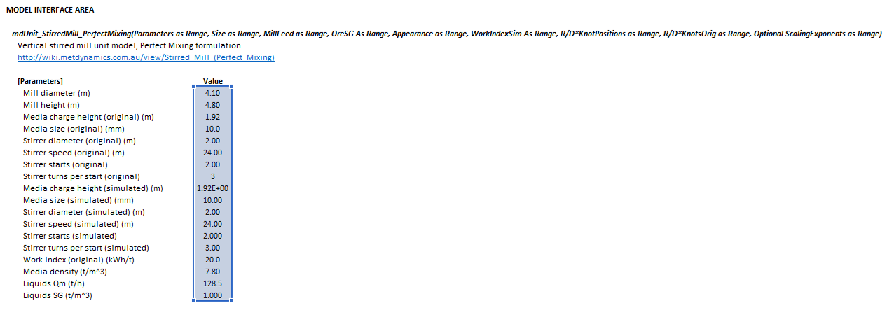
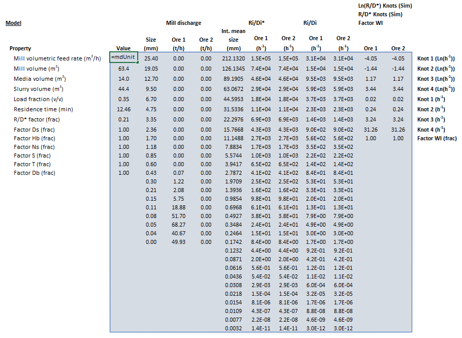
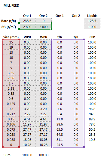
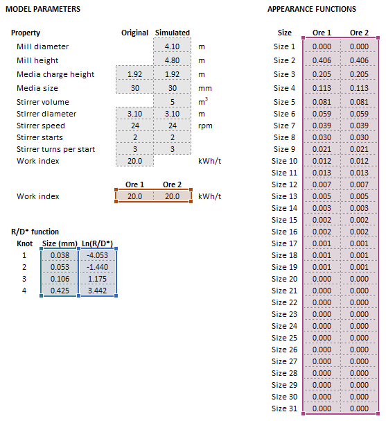
The images below show the selection of input arrays and output results in the Excel interface. | |||
{| | |||
|- style="vertical-align:top;" | |||
| [[File:StirredMillPerfectMixing2.png|left|frame|Figure 3. Example showing the selection of the '''Parameters''' (blue frame) array in Excel.]] | |||
[[File:StirredMillPerfectMixing5.png|left|frame|Figure 4. Example showing the outline of the '''Results''' (light blue frame) array in Excel.]] | |||
|| [[File:StirredMillPerfectMixing3.png|left|frame|Figure 5. Example showing the selection of the '''Size''' (red frame), '''OreSG''' (green frame) and '''MillFeed''' (purple frame).]] || [[File:StirredMillPerfectMixing4.png|left|frame|Figure 6. Example showing the selection of the '''Appearance''' (pink frame), '''R/D*KnotPositions''' (teal frame), '''R/D*KnotsOrig''' (blue frame), '''WorkIndexSim''' (red frame) arrays in Excel.]] | |||
|} | |||
== SysCAD == | |||
The SysCAD interface for steady-state (ProBal) mode is described below. For SysCAD Dynamic, see ''[[Stirred Mill (Perfect Mixing, Dynamic)]]''. | |||
{{SysCAD (Page, Mill, DLL*Mill)|PowerModels=true|MediaStrings=true}} | |||
{{SysCAD (Page, Stirred Mill, Perfect Mixing, Mill)|method=0}} | |||
{{SysCAD (Page, Ball Mill, Perfect Mixing, Ore)|method=Stirred}} | |||
{{SysCAD (Page, Stirred Mill, Perfect Mixing, Ri/Di)|method=0}} | |||
{{SysCAD (Page, Tumbling Mill, Power)|modelpage={{SysCAD (Text, UnitType Prefix)}}Mill|Nitta=true|Heath=true}} | |||
{{SysCAD (Page, Tumbling Mill, MediaStrings)|modelpage={{SysCAD (Text, UnitType Prefix)}}Mill}} | |||
{{SysCAD (Page, About)}} | |||
== See also == | |||
* [[Stirred Mill (Perfect Mixing, Dynamic)|Dynamic Perfect Mixing stirred mill model]] | |||
* [[Mill (Herbst-Fuerstenau)| Herbst-Fuerstenau mill model]] | |||
* [[Stirred Mill (Power, Nitta)]] | |||
* [[Stirred Mill (Power, Heath)]] | |||
== External links == | |||
* [https://help.syscad.net/Met_Dynamics_-_Mill Met Dynamics - Mill (help.syscad.net)] | |||
* [https://help.syscad.net/Example_-_09_Met_Dynamics_Projects#Crushing_and_Grinding_Example Crushing and Grinding Example project (help.syscad.net)] | |||
* [https://help.syscad.net/Example_-_09_Met_Dynamics_Projects#Crushing,_Grinding_and_Flotation_Example Crushing, Grinding and Flotation Example project (help.syscad.net)] | |||
== References == | == References == | ||
[[Category:Excel]] | |||
[[Category:SysCAD]] | |||
Latest revision as of 13:28, 1 May 2025
Description
This article describes an implementation of the Perfect Mixing vertical stirred mill model outlined by Napier-Munn et al. (1996).[1]
The model described here is for steady-state simulation. For dynamic simulation, see Stirred Mill (Perfect Mixing, Dynamic).
Model theory
Discharge rate
Breakage rate
Appearance function
Internal mesh series
Multi-component modelling
Excel
The Perfect Mixing stirred mill model may be invoked from the Excel formula bar with the following function call:
=mdUnit_StirredMill_PerfectMixing(Parameters as Range, Size as Range, MillFeed as Range, OreSG As Range, Appearance as Range, WorkIndexSim As Range, R/D*KnotPositions as Range, R/D*KnotsOrig as Range, Optional ScalingExponents as Range)
Invoking the function with no arguments will print Help text associated with the model, including a link to this page.
Inputs
The required inputs are defined below in matrix notation with elements corresponding to cells in Excel row ([math]\displaystyle{ i }[/math]) x column ([math]\displaystyle{ j }[/math]) format:
- [math]\displaystyle{ Parameters= \begin{bmatrix} D\text{ (m)}\\ H\text{ (m)}\\ (H_{\rm b})_{\rm Orig}\text{ (m)}\\ (D_{\rm b})_{\rm Orig}\text{ (mm)}\\ (D_{\rm s})_{\rm Orig}\text{ (m)}\\ (N_{\rm s})_{\rm Orig}\text{ (rpm)}\\ S_{\rm Orig}\\ T_{\rm Orig}\\ (H_{\rm b})_{\rm Sim}\text{ (m)}\\ (D_{\rm b})_{\rm Sim}\text{ (mm)}\\ (D_{\rm s})_{\rm Sim}\text{ (m)}\\ (N_{\rm s})_{\rm Sim}\text{ (rpm)}\\ S_{\rm Sim}\\ T_{\rm Sim}\\ {\rm WI}_{\rm Orig}\text{ (kWh/t)}\\ (Q_{\rm M,F})_{\rm L}\text{ (t/h)}\\ \rho_{\rm L}\text{ (t/m}^{\text{3}}\text{)}\\ \end{bmatrix},\;\;\;\;\;\; Size = \begin{bmatrix} d_{1}\text{ (mm)}\\ \vdots\\ d_n\text{ (mm)}\\ \end{bmatrix},\;\;\;\;\;\; MillFeed= \begin{bmatrix} (Q_{\rm M,F})_{11}\text{ (t/h)} & \dots & (Q_{\rm M,F})_{1m}\text{ (t/h)}\\ \vdots & \ddots & \vdots\\ (Q_{\rm M,F})_{n1}\text{ (t/h)} & \dots & (Q_{\rm M,F})_{nm}\text{ (t/h)}\\ \end{bmatrix},\;\;\;\;\;\; OreSG= \begin{bmatrix} (\rho_{\rm S})_{1}\text{ (t/m}^\text{3}\text{)} & \dots & (\rho_{\rm S})_m\text{ (t/m}^\text{3}\text{)}\\ \end{bmatrix} }[/math]
- [math]\displaystyle{ Appearance= \begin{bmatrix} \begin{bmatrix} A_{1}\text{ (frac)}\\ \vdots\\ A_{31}\text{ (frac)}\\ \end{bmatrix}_1 \dots \begin{bmatrix} A_{1}\text{ (frac)}\\ \vdots\\ A_{31}\text{ (frac)}\\ \end{bmatrix}_m \end{bmatrix},\;\;\;\;\;\; {\rm WI}_{\rm Sim}= \begin{bmatrix} {\rm WI}_{1}\text{ (kWh/t)} & \dots & {\rm WI}_m\text{ (kWh/t)}\\ \end{bmatrix},\;\;\;\;\;\; R/D^*KnotPositions= \begin{bmatrix} d_{1}\text{ (mm)}\\ \vdots\\ d_{k}\text{ (mm)}\\ \end{bmatrix},\;\;\;\;\;\; R/D^*KnotOrig= \begin{bmatrix} \ln\left(\frac{R}{D^*}\right)_1\\ \vdots\\ \ln\left(\frac{R}{D^*}\right)_k\\ \end{bmatrix} }[/math]
- [math]\displaystyle{ \mathit{ScalingExponents} = \begin{bmatrix} e_1\\ e_2\\ e_3\\ e_4\\ e_5\\ e_6\\ e_7\\ \end{bmatrix}^* }[/math]
where:
- [math]\displaystyle{ (Q_{\rm M,F})_{\rm L} }[/math] is the mass flow feed rate of liquids into the mill (t/h)
- [math]\displaystyle{ \rho_{\rm B} }[/math] is the Specific Gravity or density of the media in the mill (- or t/m3)
- [math]\displaystyle{ \rho_{\rm L} }[/math] is the Specific Gravity or density of liquids in the feed (- or t/m3)
- [math]\displaystyle{ m }[/math] is the number of ore types
- [math]\displaystyle{ k }[/math] is the number of breakage rate per discharge rate knots
- [math]\displaystyle{ d_i }[/math] is the size of the square mesh interval that feed mass is retained on (mm)
- [math]\displaystyle{ d_{i+1}\lt d_i\lt d_{i-1} }[/math], i.e. descending size order from top size ([math]\displaystyle{ d_{1} }[/math]) to sub mesh ([math]\displaystyle{ d_{n}=0 }[/math] mm)
- [math]\displaystyle{ Q_{\rm M,F} }[/math] is the mass flow rate of particles in the feed (t/h)
- [math]\displaystyle{ \rho_{\rm S} }[/math] is the Specific Gravity or density of solids (- or t/m3)
- [math]\displaystyle{ ^* }[/math] indicates the [math]\displaystyle{ \mathit{ScalingExponents} }[/math] array is optional, the default values are used if omitted.
Results
The results are displayed in Excel as an array corresponding to the matrix notation below:
- [math]\displaystyle{ mdUnit\_StirredMill\_PerfectMixing = \begin{bmatrix} \begin{bmatrix} Q_{\rm V}\text{ (m}^{\text{3}}\text{/h)}\\ V_{\rm Mill}\text{ (m}^{\text{3}}\text{)}\\ V_{\rm Media}\\ V_{\rm Slurry}\\ {\rm LF}\text{ (v/v)}\\ \tau\text{ (min)}\\ \text{R/D* factor (frac)}\\ f_{\rm Ds}\text{ (-)}\\ f_{\rm Hb}\text{ (-)}\\ f_{\rm Ns}\text{ (-)}\\ f_{\rm S}\text{ (-)}\\ f_{\rm T}\text{ (-)}\\ f_{\rm Db}\text{ (-)}\\ f_{\rm WI}\text{ (-)}\\ \end{bmatrix} & \begin{array}{cccccc} \begin{bmatrix} d_1\text{ (mm)}\\ \vdots\\ d_n\text{ (mm)} \end{bmatrix} & \begin{bmatrix} (Q_{\rm M,P})_{11}\text{ (t/h)} & \dots & (Q_{\rm M,P})_{1m}\text{ (t/h)}\\ \vdots & \ddots & \vdots\\ (Q_{\rm M,P})_{n1}\text{ (t/h)} & \dots & (Q_{\rm M,P})_{nm}\text{ (t/h)}\\ \end{bmatrix} & \begin{bmatrix} \bar{d}_1\text{ (mm)}\\ \vdots\\ \bar{d}_{31}\text{ (mm)}\\ \end{bmatrix} & \begin{bmatrix} \frac{R_i}{D_i^*}_{11}\left(\frac{\text{h}^\text{-1}}{\text{h}^\text{-1}}/\text{h}\right) & \dots & \frac{R_i}{D_i^*}_{1m}\left(\frac{\text{h}^\text{-1}}{\text{h}^\text{-1}}/\text{h}\right)\\ \vdots & \ddots & \vdots \\ \frac{R_i}{D_i^*}_{31,1}\left(\frac{\text{h}^\text{-1}}{\text{h}^\text{-1}}/\text{h}\right) & \dots & \frac{R_i}{D_i^*}_{31m}\left(\frac{\text{h}^\text{-1}}{\text{h}^\text{-1}}/\text{h}\right)\\ \end{bmatrix} & \begin{bmatrix} \frac{R_i}{D_i}_{11}\left(\frac{\text{h}^\text{-1}}{\text{h}^\text{-1}}\right) & \dots & \frac{R_i}{D_i}_{1m}\left(\frac{\text{h}^\text{-1}}{\text{h}^\text{-1}}\right)\\ \vdots & \ddots & \vdots \\ \frac{R_i}{D_i}_{31,1}\left(\frac{\text{h}^\text{-1}}{\text{h}^\text{-1}}\right) & \dots & \frac{R_i}{D_i}_{31m}\left(\frac{\text{h}^\text{-1}}{\text{h}^\text{-1}}\right)\\ \end{bmatrix} & \begin{bmatrix} \ln \left( \frac{R_i}{D_i} \right)_{11} & \dots & \ln \left( \frac{R_i}{D_i} \right)_{1m}\\ \vdots & \ddots & \vdots \\ \ln \left( \frac{R_i}{D_i} \right)_{k1} & \dots & \ln \left( \frac{R_i}{D_i} \right)_{km}\\ \end{bmatrix}\\ \\ & & & & & \begin{bmatrix} \left( \frac{R_i}{D_i} \right)_{11}\left(\frac{\text{h}^\text{-1}}{\text{h}^\text{-1}}\right) & \dots & \left( \frac{R_i}{D_i} \right)_{1m}\left(\frac{\text{h}^\text{-1}}{\text{h}^\text{-1}}\right)\\ \vdots & \ddots & \vdots \\ \left( \frac{R_i}{D_i} \right)_{k1}\left(\frac{\text{h}^\text{-1}}{\text{h}^\text{-1}}\right) & \dots & \left( \frac{R_i}{D_i} \right)_{km}\left(\frac{\text{h}^\text{-1}}{\text{h}^\text{-1}}\right)\\ \end{bmatrix}\\ \\ & & & & & \begin{bmatrix} (Factor_{\rm WI})_1 & \dots & (Factor_{\rm WI})_m \end{bmatrix}\\ \\ & & & & & & \\ & & & & & & \end{array} \end{bmatrix} }[/math]
where:
- [math]\displaystyle{ {\rm LF} }[/math] is the media load fraction (v/v), defined as the fraction of mill volume occupied by media, including void spaces, i.e. [math]\displaystyle{ {\rm LF} = H_{\rm b} \big/ H }[/math]
- [math]\displaystyle{ \text{R/D* factor}=D_i^*/D_i }[/math] is the discharge rate scaling factor
- [math]\displaystyle{ Q_{\rm M,P} }[/math] is the mass flow rate of particles in the mill product (t/h)
- [math]\displaystyle{ \bar{d}_i }[/math] is the geometric mean size of the internal mesh series interval that mass is retained on (mm)
Example
The images below show the selection of input arrays and output results in the Excel interface.
SysCAD
The SysCAD interface for steady-state (ProBal) mode is described below. For SysCAD Dynamic, see Stirred Mill (Perfect Mixing, Dynamic).
MD_Mill page
The first tab page in the access window will have this name.
| Tag (Long/Short) | Input / Display | Description/Calculated Variables/Options |
|---|---|---|
| Tag | Display | This name tag may be modified with the change tag option. |
| Condition | Display | OK if no errors/warnings, otherwise lists errors/warnings. |
| ConditionCount | Display | The current number of errors/warnings. If condition is OK, returns 0. |
| GeneralDescription / GenDesc | Display | This is an automatically generated description for the unit. If the user has entered text in the 'EqpDesc' field on the Info tab (see below), this will be displayed here.
If this field is blank, then SysCAD will display the unit class ID. |
| Requirements | ||
| On | CheckBox | This enables the unit. If this box is not checked, then the material will pass straight through the mill with no change to the size distribution. |
| NumParallelUnits | Input | The number of parallel, identical units to simulate:
|
| Method | Fixed Discharge | The discharge particle size distribution is user defined. Different distributions can be used for different solids. |
| AG/SAG (Variable Rates) | The Variable Rates AG/SAG mill model (steady-state or dynamic) is used to determine the mill product size distribution. Different parameters can be used for different solids. | |
| Rod Mill (Lynch) | The Lynch rod mill model is used to determine the mill product size distribution. Different parameters can be used for different solids. | |
| Ball (Perfect Mixing) | The Perfect Mixing ball mill model (steady-state or dynamic) is used to determine the mill product size distribution. Different parameters can be used for different solids. | |
| Stirred (Perfect Mixing) | The Perfect Mixing stirred mill model (steady-state or dynamic) is used to determine the mill product size distribution. Different parameters can be used for different solids. | |
| Mill (Herbst-Fuerstenau) | The Herbst-Fuerstenau model is used to determine the mill product size distribution. Different parameters can be used for different solids. | |
| PowerModels | CheckBox | Show alternative mill power model calculations on the Power page. |
| MediaStrings | CheckBox | Show media size distributions at recharge equilibrium on the MediaStrings page. |
| Options | ||
| ShowQFeed | CheckBox | QFeed and associated tab pages (eg Sp) will become visible, showing the properties of the combined feed stream. |
| ShowQProd | CheckBox | QProd and associated tab pages (eg Sp) will become visible, showing the properties of the products. |
| SizeForPassingFracCalc | Input | Size fraction for % Passing calculation. The size fraction input here will be shown in the Stream Summary section. |
| FracForPassingSizeCalc | Input | Fraction passing for Size calculation. The fraction input here will be shown in the Stream Summary section. |
| Stream Summary | ||
| MassFlow / Qm | Display | The total mass flow in each stream. |
| SolidMassFlow / SQm | Display | The Solids mass flow in each stream. |
| LiquidMassFlow / LQm | Display | The Liquid mass flow in each stream. |
| VolFlow / Qv | Display | The total Volume flow in each stream. |
| Temperature / T | Display | The Temperature of each stream. |
| Density / Rho | Display | The Density of each stream. |
| SolidFrac / Sf | Display | The Solid Fraction in each stream. |
| LiquidFrac / Lf | Display | The Liquid Fraction in each stream. |
| Passing | Display | The mass fraction passing the user-specified size (in the field SizeForPassingFracCalc) in each stream. |
| Passes | Display | The user-specified (in the field FracForPassesSizeCalc) fraction of material in each stream will pass this size fraction. |
Mill page
The Mill page is used to specify the input parameters for the mill model.
| Tag (Long/Short) | Input / Display | Description/Calculated Variables/Options |
|---|---|---|
| PerfectMixing | ||
| HelpLink | Opens a link to this page using the system default web browser. Note: Internet access is required. | |
| Stirred | ||
| MediaStringsP50 | CheckBox |
|
| UserExponents | Checkbox | Indicates whether to use user-defined values for the scaling exponents. |
| MillDiameter | Input | The inside liner diameter of the simulated mill. |
| MillHeight | Input | The height of the simulated mill. |
| MediaHeight | Input | Height of the media charge of the original and simulated mills. |
| MediaDiameter | Input | Median diameter of the media in the original and simulated mills. |
| StirrerDiameter | Input | Diameter of the stirrers of the original and simulated mills. |
| StirrerSpeed | Input | Rotational speed of the stirrers of the original and simulated mills. |
| StirrerStarts | Input | Number of starts of the (screw) stirrers of the original and simulated mills. |
| StirrerTurns | Input | Number of turns per start of the (screw) stirrers of the original and simulated mills. |
| WorkIndex | Input | Bond Ball Work Index of ore in the original mill. |
| Exponent | Input |
|
| R/DFunction | ||
| NumSplineKnots | Input | Number of spline knots for the [math]\displaystyle{ R_i/D_i^* }[/math] function. |
| Size | Input | Spline knot size positions. |
| Ln(R/D*) | Input | Values of [math]\displaystyle{ \ln R/D^* }[/math] at each spline knot position. |
| Results | ||
| MillVolume | Display | Volume inside the mill. |
| MediaVolume | Display | Volume occupied by the media in the mill, excluding void space. |
| SlurryVolume | Display | Volume of slurry in the mill, including slurry in media void space and above media charge. |
| LoadFraction | Display | Volume of media charge, including void space and excluding stirrer volume, as a fraction of mill volume, excluding stirrer volume. |
| ResidenceTime | Display | Mean residence time of slurry in the mill. |
Ore page
This page is used to define the comminution properties of SysCAD species with the size distribution quality in the project.
| Tag (Long/Short) | Input / Display | Description/Calculated Variables/Options |
|---|---|---|
| Appearance | ||
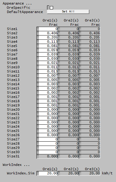
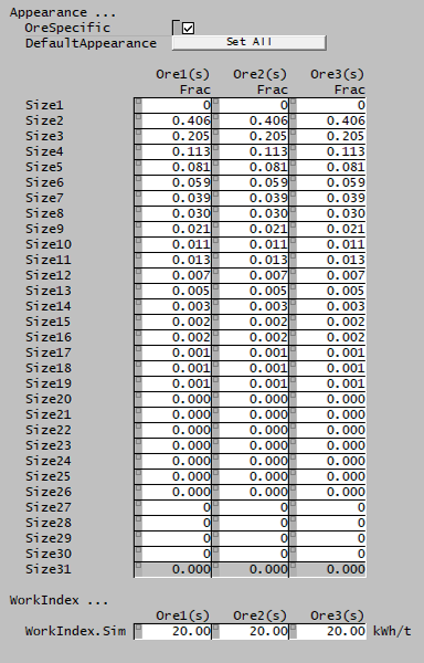
| DefaultAppearance | Sets all species to the default Kelsall Appearance function. | |
| OreSpecific | CheckBox |
|
| Appearance | Input | User-specified Appearance function data for all species with size distribution property. |
| WorkIndex | ||
| WorkIndex.Sim | Input | Bond Ball Work Index data for all species with size distribution property. |
Ri/Di page
This page displays the scaling factors and breakage rate per discharge rate for each size interval computed by the Perfect Mixing model.
| Tag (Long/Short) | Input / Display | Description/Calculated Variables/Options |
|---|---|---|
| Scaling | ||
| RDStar/RD | Display | Value of the [math]\displaystyle{ \frac{R}{D^*} \bigg/ \frac{R}{D} }[/math] factor for discharge rate scaling. |
| StirrerDiameter | Display | Value of the stirrer diameter factor for rate scaling. |
| MediaHeight | Display | Value of the media height factor for rate scaling. |
| StirrerSpeed | Display | Value of the stirrer speed factor for rate scaling. |
| StirrerStarts | Display | Value of the stirrer starts factor for rate scaling. |
| StirrerTurns | Display | Value of the stirrer turns per start factor for rate scaling. |
| MediaSize | Display | Value of the media size factor for rate scaling. |
| WorkIndex | Display | Value of the Work Index factor of each ore species for rate scaling. |
| Ri/DiStar | ||
| Size | Display | Size of each interval in internal mesh series. |
| MeanSize | Display | Geometric mean size of each interval in internal mesh series. |
| Ri/DiStar | Display | Value of normalised [math]\displaystyle{ R_i/D_i^* }[/math] rate for each size interval, for each ore species. |
| Ri/Di | ||
| Size | Display | Size of each interval in internal mesh series. |
| MeanSize | Display | Geometric mean size of each interval in internal mesh series. |
| Ri/Di | Display | Value of [math]\displaystyle{ R_i/D_i }[/math] rate for each size interval, for each ore species. |
Power page
This optional page displays the inputs and results for alternative mill power models. The page is only visible if PowerModels is selected on the MD_Mill page.
| Tag (Long/Short) | Input / Display | Description/Calculated Variables/Options |
|---|---|---|
| Power | ||
| Nitta | CheckBox | Shows inputs and results for stirred mill power calculations using the Nitta method. |
| Heath | CheckBox | Shows inputs and results for stirred mill power calculations using the Heath method. |
MediaStrings page
This page displays the inputs and results for grinding mill media string calculations. The page is only visible if MediaStrings is selected on the MD_Mill page.
About page
This page is provides product and licensing information about the Met Dynamics Models SysCAD Add-On.
| Tag (Long/Short) | Input / Display | Description/Calculated Variables/Options |
|---|---|---|
| About | ||
| HelpLink | Opens a link to the Installation and Licensing page using the system default web browser. Note: Internet access is required. | |
| Information | Copies Product and License information to the Windows clipboard. | |
| Product | ||
| Name | Display | Met Dynamics software product name |
| Version | Display | Met Dynamics software product version number. |
| BuildDate | Display | Build date and time of the Met Dynamics Models SysCAD Add-On. |
| License | ||
| File | This is used to locate a Met Dynamics software license file. | |
| Location | Display | Type of Met Dynamics software license or file name and path of license file. |
| SiteCode | Display | Unique machine identifier for license authorisation. |
| ReqdAuth | Display | Authorisation level required, MD-SysCAD Full or MD-SysCAD Runtime. |
| Status | Display | License status, LICENSE_OK indicates a valid license, other messages report licensing errors. |
| IssuedTo | Display | Only visible if Met Dynamics license file is used. Name of organisation/seat the license is authorised to. |
| ExpiryDate | Display | Only visible if Met Dynamics license file is used. License expiry date. |
| DaysLeft | Display | Only visible if Met Dynamics license file is used. Days left before the license expires. |
See also
- Dynamic Perfect Mixing stirred mill model
- Herbst-Fuerstenau mill model
- Stirred Mill (Power, Nitta)
- Stirred Mill (Power, Heath)
External links
- Met Dynamics - Mill (help.syscad.net)
- Crushing and Grinding Example project (help.syscad.net)
- Crushing, Grinding and Flotation Example project (help.syscad.net)
References
- ↑ Napier-Munn, T.J., Morrell, S., Morrison, R.D. and Kojovic, T., 1996. Mineral comminution circuits: their operation and optimisation. Julius Kruttschnitt Mineral Research Centre, Indooroopilly, QLD.
