Mass Balancing (n-Product Formula): Difference between revisions
imported>Scott.Munro m (→Excel) |
imported>Scott.Munro mNo edit summary |
||
| (2 intermediate revisions by the same user not shown) | |||
| Line 5: | Line 5: | ||
== Model theory == | == Model theory == | ||
{{Restricted content}} | |||
<hide> | |||
The ''method of mass flow errors'' is applied to estimate the solids split and recovery of multiple assayed components to an arbitrary number of product streams.{{Greet (2010)}} | The ''method of mass flow errors'' is applied to estimate the solids split and recovery of multiple assayed components to an arbitrary number of product streams.{{Greet (2010)}} | ||
| Line 11: | Line 14: | ||
Mineral compositions, particle size distributions and water fractions can be substituted in place of metal assays in the method. | Mineral compositions, particle size distributions and water fractions can be substituted in place of metal assays in the method. | ||
</hide><div class="user-show"> | |||
=== Unweighted estimates === | === Unweighted estimates === | ||
</div><hide> | |||
The solids mass flow split to each product stream is found by minimising the unweighted sum of squares of the differences between the mass flows of each assayed component in the feed and product streams, i.e. | The solids mass flow split to each product stream is found by minimising the unweighted sum of squares of the differences between the mass flows of each assayed component in the feed and product streams, i.e. | ||
| Line 38: | Line 43: | ||
:<math>R_{ij} = \dfrac{\beta_j p_{ij}}{\hat{f}_i}</math> | :<math>R_{ij} = \dfrac{\beta_j p_{ij}}{\hat{f}_i}</math> | ||
</hide><div class="user-show"> | |||
=== Weighted estimates === | === Weighted estimates === | ||
</div><hide> | |||
A weighted sum of squares for minimisation can be generated which takes into account measurement uncertainty. | A weighted sum of squares for minimisation can be generated which takes into account measurement uncertainty. | ||
| Line 49: | Line 54: | ||
where: | where: | ||
* <math>\sigma_{{\rm f}i}</math> is the standard deviation of the assay of component <math>i</math> in the feed stream | * <math>\sigma_{{\rm f}i}</math> is the absolute standard deviation of the assay of component <math>i</math> in the feed stream | ||
* <math>\sigma_{ij}</math> is the standard deviation of the assay of component <math>i</math> in product stream <math>j</math> | * <math>\sigma_{ij}</math> is the absolute standard deviation of the assay of component <math>i</math> in product stream <math>j</math> | ||
The weighted solids splits is therefore found from: | The weighted solids splits is therefore found from: | ||
| Line 57: | Line 62: | ||
and the reconstituted feed assays and component recoveries are computed as for the unweighted case. | and the reconstituted feed assays and component recoveries are computed as for the unweighted case. | ||
<!-- | <!-- | ||
=== Monte Carlo estimates === | === Monte Carlo estimates === | ||
| Line 68: | Line 74: | ||
The Monte Carlo method proceeds as follows: | The Monte Carlo method proceeds as follows: | ||
# A set of randomised assays are repeatedly drawn from probability distributions representing the uncertainly of | # A set of randomised assays are repeatedly drawn from probability distributions representing the uncertainly of each measurement. | ||
# In this implementation, the assays are assumed be normally distributed and independent. | # In this implementation, the assays are assumed be normally distributed and independent. | ||
# Solid mass splits and recoveries are computed for each randomised assay set. | # Solid mass splits and recoveries are computed for each randomised assay set. | ||
# As number of randomised draws increases, the mean values and variances of the mass splits and recoveries will approach their true values. | # As number of randomised draws increases, the mean values and variances of the mass splits and recoveries will approach their true values. | ||
--> | --> | ||
</hide><div class="user-show"> | |||
=== Additional notes === | |||
</div><hide> | |||
</hide><div class="user-show"> | |||
==== Absolute and relative standard deviations ==== | |||
</div><hide> | |||
The assay standard deviations required for the weighted estimates, (<math>\sigma_{\rm f},\sigma_{ij}</math>), are ''absolute'' standard deviations, and posses the same units as the assay measurement. | |||
However, many other literature sources quote ''relative'' standard deviations, usually as percentages, which must be converted to absolute values. For example: | |||
:<math>\sigma_{\rm fi} = \mathrm{RSD}_{\rm fi} . f_i </math> | |||
for the feed stream assays, where <math>\mathrm{RSD}</math> is the Relative Standard Deviation (frac). | |||
Care must be taken to differentiate between absolute and relative values when applying error models, e.g. the Whiten approach for particle size distributions.{{Greet (2010)}}{{Napier-Munn et al. (1996)}} | |||
</hide><div class="user-show"> | |||
==== Component assay magnitude ==== | |||
</div><hide> | |||
Component assays with larger values will tend to dominate the results of the method of mass flow errors. For example, component assays with values of thousands of parts per million will affect the solids mass split more than components with value of a fraction of a weight percent. | |||
This can be addressed as follows: | |||
* For the unweighted estimates case, the measured assay values can be scaled to more appropriate units, e.g. 100g/t rather than g/t. | |||
* For the weighted estimates case, the absolute standard deviations can be scaled to produce the same effect. | |||
The scaling factors applied in either case are arbitrary, and should be selected to reflect the relative "importance" or "confidence" of the component measurement. | |||
</hide> | |||
== Excel == | == Excel == | ||
| Line 78: | Line 115: | ||
The n-product formula may be invoked from the Excel formula bar with the following function call: | The n-product formula may be invoked from the Excel formula bar with the following function call: | ||
<syntaxhighlight lang="vb">=mdMassBal_nProductFormula(Assays as Range, Optional AbsSD as Range)</syntaxhighlight> | <syntaxhighlight lang="vb">=mdMassBal_nProductFormula(Assays as Range, Optional AbsSD as Range, Optional Transposed as Boolean = False)</syntaxhighlight> | ||
{{Excel (Text, Help, No Arguments)}} | {{Excel (Text, Help, No Arguments)}} | ||
The input parameters and calculation results are defined below in matrix notation, along with | The input parameters and calculation results are defined below in matrix notation, along with example images showing the selection of the same cells and arrays in the Excel interface. | ||
=== Default === | |||
The following default arrangement of inputs and results ranges apply when the formula argument ''Transposed'' is '''false''' or omitted: | |||
{| | {| | ||
| Line 128: | Line 169: | ||
| | | | ||
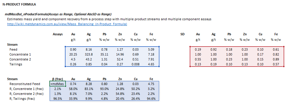
::[[File:NProductFormula3.png|frame|Figure 1. Example showing the selection of the '''Assay''' (blue frame), '''AbsSD''' (red frame), and '''Results''' (light blue frame) arrays in Excel.]] | ::[[File:NProductFormula3.png|frame|Figure 1. Example showing the selection of the '''Assay''' (blue frame), '''AbsSD''' (red frame), and '''Results''' (light blue frame) arrays in Excel.]] | ||
|} | |||
=== Transposed === | |||
The following arrangement of inputs and results ranges apply when the formula argument ''Transposed'' is '''true''': | |||
{| | |||
|- style="vertical-align:top;" | |||
| | |||
{| | |||
|- style="vertical-align:top;" | |||
| | |||
:<math> | |||
\begin{align} | |||
\mathit{Assay} & = | |||
\begin{bmatrix} | |||
f_1 & p_{11} & \cdots & p_{1n}\\ | |||
\vdots & \vdots & \ddots\\ | |||
f_m & p_{1m} & \cdots & p_{mn}\\ | |||
\end{bmatrix}\\ | |||
\\ | |||
\mathit{AbsSD} & = | |||
\begin{bmatrix} | |||
\sigma_{{\rm f} 1} & \sigma_{11} & \cdots & \sigma_{1n}\\ | |||
\vdots & \vdots & \ddots\\ | |||
\sigma_{{\rm f} m} & \sigma_{1m} & \cdots & \sigma_{mn}\\ | |||
\end{bmatrix}\\ | |||
\end{align}</math> | |||
| | |||
::<math> | |||
\begin{align} | |||
\mathit{mdMassBal\_nProductFormula} & = | |||
\begin{bmatrix} | |||
\beta_{\rm f}\text{ (frac)} & \beta_1\text{ (frac)} & \cdots & \beta_n\text{ (frac)}\\ | |||
\hat{f}_1\text{ (frac)} & R_{11}\text{ (frac)} & \cdots & R_{1n}\text{ (frac)}\\ | |||
\vdots & \vdots & \ddots & \vdots\\ | |||
\hat{f}_m\text{ (frac)} & R_{m1}\text{ (frac)} & \cdots & R_{mn}\text{ (frac)}\\ | |||
\end{bmatrix} | |||
\end{align} | |||
</math> | |||
|- style="vertical-align:top;" | |||
|colspan="2"| | |||
|} | |||
| | |||
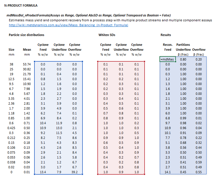
::[[File:NProductFormula4.png|frame|Figure 2. Example showing the selection of the '''Assay''' (blue frame), '''AbsSD''' (red frame), and '''Results''' (light blue frame) arrays in Excel when <math>\mathit{Transposed} = \mathrm{True}</math>.]] | |||
|} | |} | ||
Latest revision as of 08:24, 1 May 2025
Description
This article describes a methodology for estimating the solids mass split and recovery of multiple assayed components from a process step with any number of product streams.
Model theory
Unweighted estimates
Weighted estimates
Additional notes
Absolute and relative standard deviations
Component assay magnitude
Excel
The n-product formula may be invoked from the Excel formula bar with the following function call:
=mdMassBal_nProductFormula(Assays as Range, Optional AbsSD as Range, Optional Transposed as Boolean = False)
Invoking the function with no arguments will print Help text associated with the model, including a link to this page.
The input parameters and calculation results are defined below in matrix notation, along with example images showing the selection of the same cells and arrays in the Excel interface.
Default
The following default arrangement of inputs and results ranges apply when the formula argument Transposed is false or omitted:
|
| ||||
Transposed
The following arrangement of inputs and results ranges apply when the formula argument Transposed is true:
|
| ||||

