Distributions

Description

This article describes methods for estimating particle size distributions using the Gaudin-Schuhmann, Rosin-Rammler and Swebrec equations.

Model theory

Figure 1. Example particle size distributions, log-linear axes.

Figure 2. Example particle size distributions, log-log axes.

Gaudin-Schuhmann

The Gaudin-Schuhmann distribution is:

$P_{i}=\left({\dfrac {d_{i}}{k}}\right)^{a}$

where:

• $i$ is the index of the size interval, $i=\{1,2,\dots ,n\}$, $n$ is the number of size intervals
• $P_{i}$ is the cumulative fraction passing size interval $i$
• $d_{i}$ is the size of the square mesh interval that mass is retained on (mm)
• $d_{i+1}<d_{i}<d_{i-1}$, i.e. descending size order from top size ($d_{1}$) to sub mesh ($d_{n}=0$ mm)
• $k$ the Gaudin-Schuhmann size parameter (mm)
• $a$ the Gaudin-Schuhmann distribution parameter

Rosin-Rammler

The Rosin-Rammler distribution is:

$P_{i}=\exp \left[-\left({\dfrac {d_{i}}{x^{1}}}\right)^{b}\right]$

where:

• $i$ is the index of the size interval, $i=\{1,2,\dots ,n\}$, $n$ is the number of size intervals
• $P_{i}$ is the cumulative fraction passing size interval $i$
• $d_{i}$ is the size of the square mesh interval that mass is retained on (mm)
• $d_{i+1}<d_{i}<d_{i-1}$, i.e. descending size order from top size ($d_{1}$) to sub mesh ($d_{n}=0$ mm)
• $x^{1}$ is the Rosin-Rammler size parameter (mm)
• $b$ is the Rosin-Rammler distribution parameter

Swebrec

The basic three-parameter Swebrec function is:

$P_{i}={\dfrac {1}{1+\left[{\dfrac {\ln \left({\dfrac {x_{\rm {max}}}{d_{i}}}\right)}{\ln \left({\dfrac {x_{\rm {max}}}{x_{50}}}\right)}}\right]^{b}}}$

where:

• $i$ is the index of the size interval, $i=\{1,2,\dots ,n\}$, $n$ is the number of size intervals
• $P_{i}$ is the cumulative fraction passing size interval $i$
• $d_{i}$ is the size of the square mesh interval that mass is retained on (mm)
• $d_{i+1}<d_{i}<d_{i-1}$, i.e. descending size order from top size ($d_{1}$) to sub mesh ($d_{n}=0$ mm)
• $x_{\rm {Max}}$ is the maximum (top) size of the distribution (mm)
• $x_{50}$ is the mean size (passing 50%) of the distribution (mm)
• $b$ is a curve-undulation exponent

The extended five-parameter Swebrec function is:

$P_{i}={\dfrac {1}{1+a\left[{\dfrac {\ln \left({\dfrac {x_{\rm {max}}}{d_{i}}}\right)}{\ln \left({\dfrac {x_{\rm {max}}}{x_{50}}}\right)}}\right]^{b}+(1-a)\left[{\dfrac {\left({\dfrac {x_{\rm {max}}}{d_{i}}}-1\right)}{\left({\dfrac {x_{\rm {max}}}{x_{50}}}-1\right)}}\right]^{c}}}$

where $a$ is a proportion parameter and $c$ is an undulation exponent.

Excel

Gaudin-Schuhmann

The Gaudin-Schuhmann distribution may be invoked from the Excel formula bar with the following function calls:

=mdDist_GaudinSchuhmann(Size as Range, k as Double, m as Double)

Invoking the function with no arguments will print Help text associated with the model, including a link to this page.

The input parameters and calculation results are defined below in matrix notation, along with an example image showing the selection of the same cells and arrays in the Excel interface:

${\begin{aligned}{\mathit {Size}}&={\begin{bmatrix}d_{1}{\text{ (mm)}}\\\vdots \\d_{n}{\text{ (mm)}}\\\end{bmatrix}}\\\\{\mathit {k}}&={\big [}k{\text{ (mm)}}{\big ]}\\\\{\mathit {a}}&={\big [}a{\big ]}\end{aligned}}$ ${\begin{aligned}{\mathit {mdDist\_GaudinSchuhmann}}&={\begin{bmatrix}P_{1}{\text{ (frac)}}\\\vdots \\P_{n}{\text{ (frac)}}\\\end{bmatrix}}\end{aligned}}$

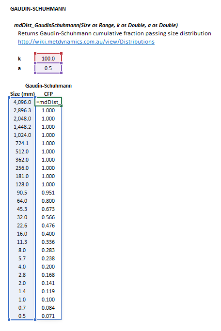Figure 3. Example showing the selection of the Size (blue frame), k (red frame), a (purple frame) and Results (light blue frame) arrays in Excel.

Rosin-Rammler

The Rosin-Rammler distribution may be invoked from the Excel formula bar with the following function calls:

=mdDist_RosinRammler(Size as Range, x1 as Double, b as Double)

Invoking the function with no arguments will print Help text associated with the model, including a link to this page.

The input parameters and calculation results are defined below in matrix notation, along with an example image showing the selection of the same cells and arrays in the Excel interface:

${\begin{aligned}{\mathit {Size}}&={\begin{bmatrix}d_{1}{\text{ (mm)}}\\\vdots \\d_{n}{\text{ (mm)}}\\\end{bmatrix}}\\\\{\mathit {x1}}&={\big [}x^{1}{\text{ (mm)}}{\big ]}\\\\{\mathit {b}}&={\big [}b{\big ]}\end{aligned}}$ ${\begin{aligned}{\mathit {mdDist\_RosinRammler}}&={\begin{bmatrix}P_{1}{\text{ (frac)}}\\\vdots \\P_{n}{\text{ (frac)}}\\\end{bmatrix}}\end{aligned}}$ where: $d_{i}$ is the size of the square mesh interval that feed mass is retained on (mm) $d_{i+1}<d_{i}<d_{i-1}$, i.e. descending size order from top size ($d_{1}$) to sub mesh ($d_{n}=0$ mm)

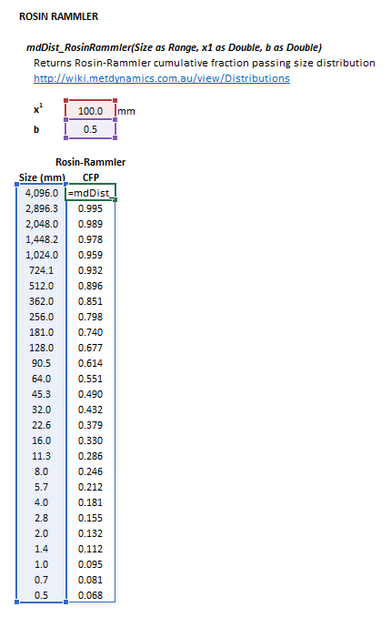Figure 4. Example showing the selection of the Size (blue frame), x1 (red frame), b (purple frame) and Results (light blue frame) arrays in Excel.

Swebrec

The Swebrec distribution may be invoked from the Excel formula bar with the following function calls:

=mdDist_Swebrec(Size as Range, xMax as Double, x50 as Double, b as Double, Optional a as Double = 1, Optional c as Double = 0)

Invoking the function with no arguments will print Help text associated with the model, including a link to this page.

The input parameters and calculation results are defined below in matrix notation, along with an example image showing the selection of the same cells and arrays in the Excel interface:

${\begin{aligned}{\mathit {Size}}&={\begin{bmatrix}d_{1}{\text{ (mm)}}\\\vdots \\d_{n}{\text{ (mm)}}\\\end{bmatrix}}\\\\{\mathit {xMax}}&={\big [}x_{\rm {Max}}{\text{ (mm)}}{\big ]}\\\\{\mathit {x50}}&={\big [}x_{50}{\text{ (mm)}}{\big ]}\\\\{\mathit {b}}&={\big [}b{\big ]}\\\\{\mathit {a}}&={\big [}a{\big ]}^{*}\\\\{\mathit {c}}&={\big [}c{\big ]}^{*}\end{aligned}}$ ${\begin{aligned}{\mathit {mdDist\_Swebrec}}&={\begin{bmatrix}P_{1}{\text{ (frac)}}\\\vdots \\P_{n}{\text{ (frac)}}\\\end{bmatrix}}\end{aligned}}$ where $^{*}$ represents optional parameters. Omitting both optional parameters will invoke the three-parameter Swebrec function, otherwise the five-parameter version is used.

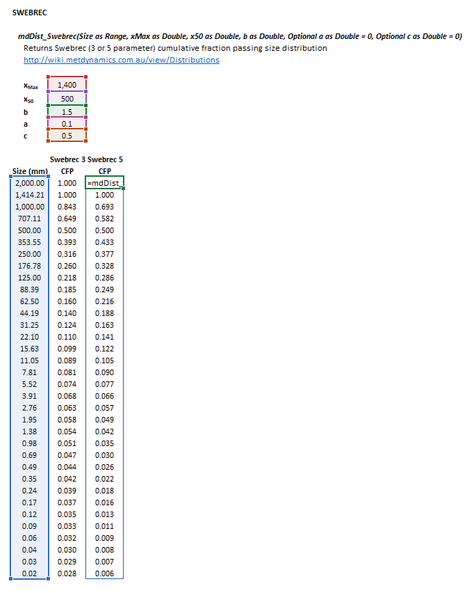Figure 5. Example showing the selection of the Size (blue frame), xMax (red frame), x50 (purple frame), b (green frame),a (pink frame), c (brown frame) and Results (light blue frame) arrays in Excel.

References

- ↑ Gupta, A. and Yan, D.S., 2016. Mineral processing design and operations: an introduction. Elsevier.
- ↑ Ouchterlony, F., 2005. The Swebrec© function: linking fragmentation by blasting and crushing. Mining Technology, 114(1), pp.29-44.