Gravity Classifier (Plitt-Flintoff)

Description

This article describes a model of gravity classifiers proposed by Plitt and Flintoff (1985).

Gravity classifiers use the differential settling velocity of particles in a pool to separate feed pulp into coarse and fine product streams.

Mechanical gravity classifiers use a mechanical action to both agitate pulp in the pool and convey the gravity-settled coarse particles away from the machine and the remaining fine particles in the overflow. Examples of mechanical gravity classifiers include spiral, rake and bowl machines.

Non-mechanical gravity classifiers rely on free or hindered settling against a rising current and draw settled coarse particles through an underflow spigot. Finer particles report to the overflow. Examples of non-mechanical gravity classifiers include devices variously referred to as hydraulic classifiers, elutriators, hydrospearators, hydrosizers, upcurrent classifiers, teeter-bed separators, hindered-bed separators, or cone classifiers.

Model theory

Figure 1. Example partition curve predicted by the Plitt-Flintoff gravity classifier model.

Plitt and Flintoff proposed a model that describes the classification of particles based on a consideration of settling velocity and flow conditions in gravity classification devices.

Classification

Plitt and Flintoff's formulation applies the Reid-Plitt (1971) efficiency curve to describe the classification of particles by size.

The Reid-Plitt expression for corrected partition to underflow, $E_{\rm {uc}}$ (frac), is:

$E_{\rm {uc}}({\bar {d}}_{i})=1-\exp \left[-\ln 2\left({\dfrac {{\bar {d}}_{i}}{d_{50{\rm {c}}}}}\right)^{m}\right]$

where:

• $i$ is the index of the size interval, $i=\{1,2,\dots ,n\}$, $n$ is the number of size intervals
• ${\bar {d}}_{i}$ is the geometric mean size of particles in size interval $i$ (mm)
• $d_{\rm {50c}}$ is the corrected size at which 50% of the particle mass reports to underflow and 50% to overflow (mm)
• $m$ is the sharpness parameter that determines the steepness of the partition curve (-)

The actual partition to underflow , $E_{\rm {ua}}$ (frac), is computed as:

$E_{\rm {ua}}({\bar {d}}_{i})=E_{\rm {uc}}({\bar {d}}_{i})+R_{\rm {f}}(1-E_{\rm {uc}}({\bar {d}}_{i}))$

where $R_{\rm {f}}$ is the fraction of fines and/or feed liquids split to the underflow (frac).

Determination of the corrected cut size ($d_{\rm {50c}}$) and water recovery ($R_{\rm {f}}$) terms of the Reid-Plitt equation are described below.

The value of the sharpness parameter, $m$, can be specified for a given application, or estimated as described below.

Corrected cut size

Plitt and Flintoff assume the corrected cut size ($d_{\rm {50c}}$) is the size of a particle which has a settling velocity equal to the mean upward rising velocity of pulp, $v$ (m/h), i.e.:

$v={\dfrac {Q_{\rm {o}}}{A}}={\dfrac {48g{d_{\rm {50c}}}^{2}(\rho _{\rm {S}}-\rho _{\rm {Eff}})}{\alpha \left(2{\left({\dfrac {d_{\rm {50c}}}{10}}\right)}^{\frac {3}{2}}{\sqrt {\dfrac {100g\rho _{\rm {S}}\rho _{\rm {Eff}}}{3}}}+10{\sqrt {48}}\beta \mu \right)}}$

where:

• $Q_{\rm {o}}$ is the volumetric flow rate of pulp in the overflow (m³/h)
• $A$ is the effective settling pool area of the classifier (m²)
• $\rho _{\rm {S}}$ is the density of solids (t/m³)
• $g$ is acceleration due to gravity (m/s²)

The effective density of slurry in the classifier, $\rho _{\rm {Eff}}$ (t/m³), is assumed to be the mean of the feed slurry density, $\rho _{\rm {F}}$ (t/m³), and overflow slurry density, $\rho _{\rm {OF}}$ (t/m³), i.e.:

$\rho _{\rm {Eff}}={\dfrac {\rho _{F}+\rho _{OF}}{2}}$

The apparent viscosity of slurry in the classifier, $\mu$ (Pa.s), is estimated by the classical Krieger-Dougherty (1959) equation:

$\mu =\mu _{\rm {0}}\left(1-{\dfrac {\phi _{\rm {Eff}}}{\phi _{\rm {m}}}}\right)^{-k\phi _{\rm {m}}}$

where:

• $\mu _{0}$ is the viscosity of the carrier fluid, i.e. water (Pa.s)
• $\phi _{\rm {m}}$ is maximum packing fraction of particles (v/v), assumed to be 0.64
• $k$ is a particle shape constant, assumed to be 2.5

The effective volume solids fraction in the classier, $\phi _{\rm {Eff}}$ (v/v), is assumed to be the mean of the feed solids volume fraction, $\phi _{\rm {F}}$ (v/v), and the overflow solids volume fraction, $\phi _{\rm {OF}}$ (v/v), i.e.:

$\phi _{\rm {Eff}}={\dfrac {\phi _{F}+\phi _{\rm {OF}}}{2}}$

The parameters $\alpha$ and $\beta$ are related to the particle shape, as shown in Table 1.

Table 1. Particle shape types

Index	Particle shape	Example mineral	${\boldsymbol {\alpha }}$	${\boldsymbol {\beta }}$
0	Spheres		0.942	3.03
1	Perfect cubes	Galena, sylvite	1.038	3.01
2	Conchoidal fracture	Quartz	1.022	4.008
3	Dodecahedral	Sphalerite	1.05	5.9
4	Plates 10x thickness		2.43	4.7
5	Plates 100x thickness	Mica	7.69	12.29
6	Irregular fracture	Arsenopyrite	1.00	12.98

The $d_{\rm {50c}}$ term is implicit in the settling velocity equation. Therefore a numerical root-finding algorithm is applied to approximate the value of $d_{\rm {50c}}$ for a given settling velocity and pulp conditions.

Water recovery

The Plitt and Flintoff model requires the volume fraction of solids in the underflow, $\phi _{\rm {UF}}$ (v/v), to be specified as an input.

The recovery of feed water to the underflow, $R_{\rm {f}}$, is thus a function of the recovery of solids to the underflow, which is in turn determined by the Reid-Plitt classification equation.

The Reid-Plitt classification equation itself features the $R_{\rm {f}}$ term, and therefore an iterative scheme is required to fully compute the Plitt and Flintoff model.

Sharpness estimation

Plitt and Flintoff suggest using the following relationship to estimate values of $m$, the separation sharpness:

$m={\begin{cases}{\dfrac {1.57}{\ln {\sqrt {\dfrac {\ln \left({\dfrac {3}{S}}\right)}{\ln \left({\dfrac {1}{3S}}\right)}}}}}&S<{\dfrac {1}{3}}\\0&S\geq {\dfrac {1}{3}}\end{cases}}$

where $S$ is the ratio of volumetric flowrates of pulp in the underflow (sands) and overflow streams, i.e. $S={\frac {Q_{\rm {V,UF}}}{Q_{\rm {V,OF}}}}$.

Plitt (1971) found the value of $m$ was in the range of 1 - 3.8 for classifiers. As such, the sharpness estimation above may not be appropriate for larger values of $S$, depending on the application. User caution is recommended.

Density-specific classification

Plitt and Flintoff's original model formulation purposely assumed that a mixture of particles of differing densities could be represented by a singular solid density value ($\rho _{\rm {S}}$).

This implementation can retain Plitt and Flintoff singular density value assumption, or compute classification curves separately for each density class, $(\rho _{\rm {S}})_{j}$ (t/m³), where $j=\{1,2,\dots ,p\}$ and $p$ is the number of density classes (or ore types, minerals etc).

Coarse solids removal capacity

If the computed mass flowrate of solids to the underflow stream, $(Q_{\rm {M,UF}})_{\rm {S}}$ (t/h), exceeds the solids removal capacity of the classifier, $(Q_{\rm {M,UF}})_{\rm {S}}^{\rm {Max}}$ (t/h), the ${d_{\rm {50c}}}$ value is increased by a small fraction. This process repeats until the underflow mass flowrate of solids is less than the removal capacity, i.e.

$({d_{\rm {50c}}})_{n+1}=1.05\cdot {d_{\rm {50c}}}_{n},{\text{ while }}(Q_{\rm {M,UF}})_{\rm {S}}>(Q_{\rm {M,UF}})_{\rm {S}}^{\rm {Max}}$

This action simulates a buildup of solids in the classifier which effectively reduces the settling pool area, driving up the cut size.

Sands solid content

Plitt and Flintoff provide the following table as a guide to the volume fraction of solids that may be expected from a classifier with a given cut size:

Table 2. Sands solids content (after Plitt and Flintoff, 1985)

${\boldsymbol {d_{\rm {50c}}}}$ (μm)	Volume fraction solids (% v/v)
600	57-60
420	53-57
300	52-54
210	53
150	52
105	51
74	49
Hydroseparators	20-40

Partition metrics

Several metrics are provided to characterise the partition curve.

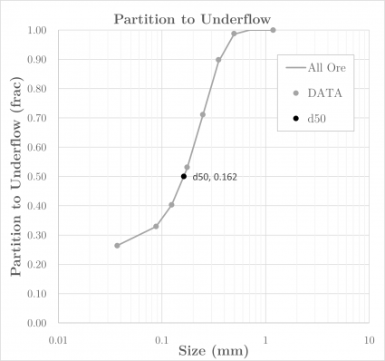
The $d_{50}$, also known as the cut or separation size, is defined as the size of a particle which has an even (50%) chance of appearing in either the underflow or overflow stream. The $d_{50}$ size is estimated via a log-linear interpolation of geometric mean size ($\ln {\bar {d}}$) against the uncorrected partition to underflow of all solids in the feed.

The Ecart Probable, or $E_{\rm {p}}$, is a measure of the deviation of a partition curve from a perfect separation, and is typically defined for size classification as:

$E_{\rm {p}}={\dfrac {d_{75}-d_{25}}{2}}$

where $d_{75}$ and $d_{25}$ are the sizes of particles which have a 75% and 25% probability, respectively, of appearing in the underflow stream. The $d_{75}$ and $d_{25}$ sizes are estimated by log-linear interpolation of geometric mean size against the uncorrected partition to underflow of all solids in the feed.

The Imperfection, $I$, is a normalised measure of the sharpness of separation, which is suggested to be independent of the magnitude of the $d_{50}$, and is typically defined for size classification as:

$I={\dfrac {E_{\rm {p}}}{d_{50}}}={\dfrac {d_{75}-d_{25}}{2d_{50}}}$

Excel

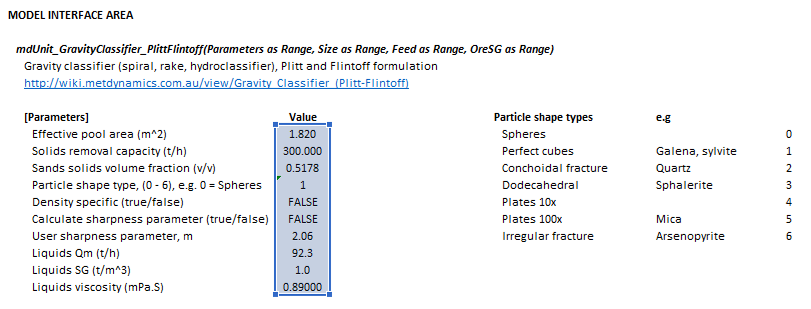
The Plitt-Flintoff gravity classifier model may be invoked from the Excel formula bar with the following function call:

=mdUnit_GravityClassifier_PlittFlintoff(Parameters as Range, Size as Range, Feed as Range, OreSG as Range)

Invoking the function with no arguments will print Help text associated with the model, including a link to this page.

Inputs

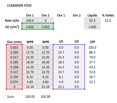
The required inputs are defined below in matrix notation with elements corresponding to cells in Excel row ($i$) x column ($j$) format:

${\mathit {Parameters}}={\begin{bmatrix}A{\text{ (m}}^{2}{\text{)}}\\(Q_{\rm {M,UF}})_{\rm {S}}^{\rm {Max}}{\text{ (t/h)}}\\\phi _{\rm {UF}}{\text{ (v/v)}}\\{\text{ Particle shape type (0-6)}}\\{\text{ Density-specific (True/False)}}\\{\text{ Calculate sharpness (True/False)}}\\{\text{ User }}m{\text{ (-)}}\\(Q_{\rm {M,F}})_{\rm {L}}{\text{ (t/h)}}\\\rho _{\rm {L}}{\text{ (t/m}}^{\text{3}}{\text{)}}\\\mu _{0}{\text{ (mPa.S)}}\\\end{bmatrix}},\;\;\;\;\;\;{\mathit {Size}}={\begin{bmatrix}d_{1}{\text{ (mm)}}\\\vdots \\d_{n}{\text{ (mm)}}\\\end{bmatrix}},\;\;\;\;\;\;{\mathit {Feed}}={\begin{bmatrix}(Q_{\rm {M,F}})_{11}{\text{ (t/h)}}&\dots &(Q_{\rm {M,F}})_{1p}{\text{ (t/h)}}\\\vdots &\ddots &\vdots \\(Q_{\rm {M,F}})_{n1}{\text{ (t/h)}}&\dots &(Q_{\rm {M,F}})_{np}{\text{ (t/h)}}\\\end{bmatrix}},\;\;\;\;\;\;{\mathit {OreSG}}={\begin{bmatrix}(\rho _{\rm {S}})_{1}{\text{ (t/m}}^{\text{3}}{\text{)}}&\dots &(\rho _{\rm {S}})_{p}{\text{ (t/m}}^{\text{3}}{\text{)}}\\\end{bmatrix}}$

where:

• ${\text{Particle shape type}}$ is the index to the particle shape factors in Table 1 (0-6)
• ${\text{Density-specific}}$ indicates whether to compute classification separately for each solids density class (True) or use a singular representative solids density (False)
• ${\text{Calculate sharpness}}$ indicates whether to estimate the sharpness of separation ($m$) (True) or apply a user-specified value (False)
• ${\text{User }}m$ is a user-specified value of the sharpness of separation ($m$) which is applied if ${\text{Calculate sharpness}}$ is False and ignored otherwise (-)
• $d_{i}$ is the size of the square mesh interval that feed mass is retained on (mm)
• $Q_{\rm {M,F}}$ is feed solids mass flow rate by size and ore type (t/h)
• $(Q_{\rm {M,F}})_{\rm {L}}$ is the mass flow feed rate of liquids into the classifier (t/h)

Results

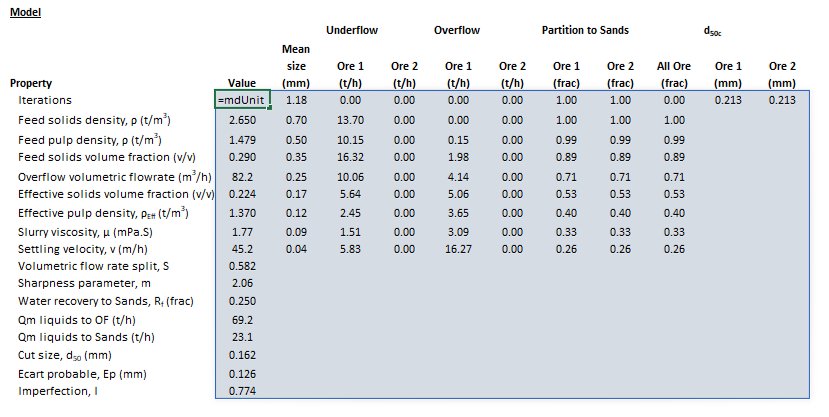
The results are displayed in Excel as an array corresponding to the matrix notation below:

${\mathit {mdUnit\_GravityClassifier\_PlittFlintoff}}={\begin{bmatrix}{\begin{bmatrix}{\text{Iterations}}\\\rho _{\rm {S}}{\text{ (t/m}}^{3}{\text{)}}\\\rho _{\rm {F}}{\text{ (t/m}}^{3}{\text{)}}\\\phi _{\rm {F}}{\text{ (v/v)}}\\Q_{\rm {o}}{\text{ (m}}^{3}{\text{/h)}}\\\phi _{\rm {Eff}}{\text{ (v/v)}}\\\rho _{\rm {Eff}}{\text{ (t/m}}^{3}{\text{)}}\\\mu {\text{ (mPa.S)}}\\v{\text{ (m/h)}}\\S{\text{ (-)}}\\m{\text{ (-)}}\\R_{\rm {f}}{\text{ (frac)}}\\(Q_{\rm {M,OF}})_{\rm {L}}{\text{ (t/h)}}\\(Q_{\rm {M,UF}})_{\rm {L}}{\text{ (t/h)}}\\d_{50}{\text{ (mm)}}\\E_{\rm {p}}{\text{ (mm)}}\\I\\\end{bmatrix}}{\begin{array}{cccccc}{\begin{bmatrix}{\bar {d}}_{1}{\text{ (mm)}}\\\vdots \\{\bar {d}}_{n}{\text{ (mm)}}\end{bmatrix}}&{\begin{bmatrix}(Q_{\rm {M,UF}})_{11}{\text{ (t/h)}}&\dots &(Q_{\rm {M,UF}})_{1p}{\text{ (t/h)}}\\\vdots &\ddots &\vdots \\(Q_{\rm {M,UF}})_{n1}{\text{ (t/h)}}&\dots &(Q_{\rm {M,UF}})_{np}{\text{ (t/h)}}\\\end{bmatrix}}&{\begin{bmatrix}(Q_{\rm {M,OF}})_{11}{\text{ (t/h)}}&\dots &(Q_{\rm {M,OF}})_{1p}{\text{ (t/h)}}\\\vdots &\ddots &\vdots \\(Q_{\rm {M,OF}})_{n1}{\text{ (t/h)}}&\dots &(Q_{\rm {M,OF}})_{np}{\text{ (t/h)}}\\\end{bmatrix}}&{\begin{bmatrix}(E_{\rm {ua}})_{11}{\text{ (frac)}}&\dots &(E_{\rm {ua}})_{1p}{\text{ (frac)}}\\\vdots &\ddots &\vdots \\(E_{\rm {ua}})_{n1}{\text{ (frac)}}&\dots &(E_{\rm {ua}})_{np}{\text{ (frac)}}\\\end{bmatrix}}&{\begin{bmatrix}(P_{\rm {UF}})_{1,{\rm {All}}}\\\vdots \\(P_{\rm {UF}})_{n,{\rm {All}}}\\\end{bmatrix}}&{\begin{bmatrix}(d_{\rm {50c}})_{1}&\dots &(d_{\rm {50c}})_{p}\\\end{bmatrix}}\\\\\\\\\\\\\\\\\\\\\\\\\\\\\\\\\end{array}}\end{bmatrix}}$

where:

• ${\text{Iterations}}$ is the number of iterations required to converge the Plitt-Flintoff model
• $(Q_{\rm {M,OF}})_{\rm {L}}$ is the mass flow rate of liquids to the overflow stream (t/h)
• $(Q_{\rm {M,UF}})_{\rm {L}}$ is the mass flow rate of liquids to the underflow stream (t/h)
• $Q_{\rm {M,UF}}$ is mass flow rate of solids to the underflow stream (t/h)
• $Q_{\rm {M,OF}}$ is mass flow rate of solids to the overflow stream (t/h)
• $(P_{\rm {UF}})_{i,{\rm {All}}}$ is the actual partition of all particles of size $i$ to the underflow stream, computed as ${\frac {\sum _{j=1}^{p}(Q_{\rm {M,UF}})_{ij}}{\sum _{j=1}^{p}(Q_{\rm {M,F}})_{ij}}}$ (frac)

Example

The images below show the selection of input arrays and output results in the Excel interface.

Figure 2. Example showing the selection of the Parameters (blue frame) array in Excel.	Figure 3. Example showing the selection of the Size (red frame), Feed (purple frame) and OreSG (green frame) arrays in Excel.
Figure 4. Example showing the outline of the Results (light blue frame) array in Excel.

SysCAD

The sections and variable names used in the SysCAD interface are described in detail in the following tables.

MD_Classifier page

The first tab page in the access window will have this name.

Tag (Long/Short)	Input / Display	Description/Calculated Variables/Options
Tag	Display	This name tag may be modified with the change tag option.
Condition	Display	OK if no errors/warnings, otherwise lists errors/warnings.
ConditionCount	Display	The current number of errors/warnings. If condition is OK, returns 0.
GeneralDescription / GenDesc	Display	This is an automatically generated description for the unit. If the user has entered text in the 'EqpDesc' field on the Info tab (see below), this will be displayed here. If this field is blank, then SysCAD will display the unit class ID.
Requirements
On	CheckBox	This enables the unit. If this box is not checked, then the MassFracToUF option appears below.
MassFracToUF	Input	Only appears if the On field above is not checked. Specifies the fraction of feed mass that reports to the underflow stream when the model is off.
NumParallelUnits	Input	The number of parallel, identical units to simulate: Feed is divided by the number of parallel units before being sent to the unit model. Unit model products are multiplied back by the same value and returned to the SysCAD product streams. All unit model result values are shown per parallel unit.
Method	Partition (User)	The partition to underflow for each size interval is defined by the user. Different values can be used for different solids.
	Partition (Reid-Plitt)	The partition to underflow for each size interval is defined by a Reid-Plitt efficiency curve. Different parameters can be used for different solids.
	Partition (Whiten-Beta)	The partition to underflow for each size interval is defined by a Whiten-Beta efficiency curve. Different parameters can be used for different solids.
	Air Classifier (Altun)	The Altun air classifier model is used to determine the partition of solids to underflow for each size interval.
	Gravity (Plitt-Flintoff)	The Plitt-Flintoff gravity classifier model is used to determine the partition of solids to underflow for each size interval.
Options
ShowQFeed	CheckBox	QFeed and associated tab pages (eg Sp) will become visible, showing the properties of the combined feed stream.
ShowQOF	CheckBox	QOF and associated tab pages (eg Sp) will become visible, showing the properties of the overflow stream.
ShowQUF	CheckBox	QUF and associated tab pages (eg Sp) will become visible, showing the properties of the underflow stream.
SizeForPassingFracCalc	Input	Size fraction for % Passing calculation. The size fraction input here will be shown in the Stream Summary section.
FracForPassingSizeCalc	Input	Fraction passing for Size calculation. The fraction input here will be shown in the Stream Summary section.
Stream Summary
MassFlow / Qm	Display	The total mass flow in each stream.
SolidMassFlow / SQm	Display	The Solids mass flow in each stream.
LiquidMassFlow / LQm	Display	The Liquid mass flow in each stream.
VolFlow / Qv	Display	The total Volume flow in each stream.
Temperature / T	Display	The Temperature of each stream.
Density / Rho	Display	The Density of each stream.
SolidFrac / Sf	Display	The Solid Fraction in each stream.
LiquidFrac / Lf	Display	The Liquid Fraction in each stream.
Passing	Display	The mass fraction passing the user-specified size (in the field SizeForPassingFracCalc) in each stream.
Passes	Display	The user-specified (in the field FracForPassesSizeCalc) fraction of material in each stream will pass this size fraction.

Classifier page

The Classifier page is used to specify the input parameters for the classifier model.

Tag (Long/Short)	Input / Display	Description/Calculated Variables/Options
PlittFlintoff
HelpLink		Opens a link to this page using the system default web browser. Note: Internet access is required.
Parameters
EffPoolArea / A	Input	Effective pool area
SolidsRemovalCapacity	Input	Maximum coarse solids removal capacity of the classifier
SandsSolVolFrac / UF.Svf	Input	Volume fraction of solids in the sands (underflow) stream
ParticleShape	Spheres	Particles are spherical.
	Perfect cubes	Particles are perfect cubes.
	Conchoidal fracture	Particles shapes are due to conchoidal fracture.
	Dodecahedral	Particles are dodecahedral
	Plates 10x	Particles are plates with length 10x width.
	Plates 100x	Particles are plates with length 100x width.
	Irregular fracture	Particles shapes are due to irregular fracture.
DensitySpecific	CheckBox	Indicates whether to determine classification per species.
CalculateSharpness	CheckBox	Indicates whether to estimate sharpness based on volume split or apply user-specific value.
UserSharpness / User_m	Input	User-specified value of sharpness. Only visible if CalculateSharpness is not selected.
Liquids
LiquidsSeparMethod	Split To UF (User)	Liquids are split to underflow by a user-defined fraction of liquids in the feed.
	Split To UF (Model)	Liquids are split to underflow by a fraction computed by the associated model.
	UF Solids Fraction	Sufficient liquids mass is recovered to the underflow stream to yield the user-defined underflow solids mass fraction value (if possible).
	UF Liquids Fraction	Sufficient liquids mass is recovered to the underflow stream to yield the user-defined underflow liquids mass fraction value (if possible).
UFSolidsFracReqd / UF.SfReqd	Input	Required value of the mass fraction of solids in the underflow stream. Only visible if UF Solids Fraction is selected.
UFLiquidsFracReqd / UF.LfReqd	Input	Required value of the mass fraction of liquids in the underflow stream. Only visible if UF Liquids Fraction is selected.
LiqSplitToUF / UF.LiqSplit	Input/Display	The fraction of liquids recovered to underflow.
Results
Iterations	Display	Number of internal iterations required to converge the Plitt-Flintoff model.
Feed.SolidDensity / Feed.SRho	Display	Density of solids in the feed stream
Feed.Density / Feed.Rho	Display	Density of slurry in the feed stream
Feed.SolidVolFrac / Feed.Svf	Display	Volume fraction of solids in the feed stream
Overflow.VolFlow / OF.Qv	Display	Volumetric flowrate of slurry in the overflow stream.
EffSolVolFrac / Eff.Svf	Display	Effective volume fraction of solids in the classifier.
EffDensity / Eff.SRho	Display	Effective density of solids in the classifier.
SlurryViscosity / mu	Display	Apparent viscosity of slurry in the classifier.
SettlingVelocity / v	Display	Settling velocity in the classifier.
VolFlowSplit / S	Display	Ratio of volumetric flow rate of slurry in the underflow to the volumetric flow rate of slurry in the overflow.
Sharpness / m	Display	Sharpness of separation in the Reid-Plitt expression.
Rf	Display	Fraction of feed liquids recovered to underflow stream.
d50	Display	The separation size, d50, of all solid particles in the feed.
EcartProbable / Ep	Display	The value of the Ecart Probable of the separation.
Imperfection / I	Display	The value of the Imperfection of the separation.
d50c	Display	Value of the corrected d50c, per species.

Partition page

The Partition page is used to specify or display the partition by species and size values.

Tag (Long/Short)	Input / Display	Description/Calculated Variables/Options
Distribution
Name	Display	Shows the name of the SysCAD Size Distribution (PSD) quality associated with the feed stream.
IntervalCount	Display	Shows the number of size intervals in the SysCAD Size Distribution (PSD) quality associated with the feed stream.
SpWithPSDCount	Display	Shows the number of species in the feed stream assigned with the SysCAD Size Distribution (PSD) quality.
Partition
Method	Model/User	Select model-calculated or user-defined partition to separate each solids species type.
Density	Display	Density of each solid species.
Size	Display	Size of each interval in mesh series.
MeanSize	Display	Geometric mean size of each interval in mesh series.
All (All column)	Display	Actual overall partition to underflow of all solid species, for each size interval. Excludes solid species not present in the classifier feed.
Partition	Display	Partition to underflow for each size interval, in each solid species, as determined by the selected model or user defined value. Note: These values are displayed regardless of whether the solid species is present in the classifier feed or not.
All (All row, All column)	Display	Displays the actual, total, partition of all solids with a particle size distribution property in the feed to underflow. Excludes solid species not present in the classifier feed.
All (All row, per species)	Display	Actual overall partition to underflow for each solid species, for all size intervals in that species. Excludes solid species not present in the classifier feed.

About page

This page is provides product and licensing information about the Met Dynamics Models SysCAD Add-On.

Tag (Long/Short)	Input / Display	Description/Calculated Variables/Options
About
HelpLink		Opens a link to the Installation and Licensing page using the system default web browser. Note: Internet access is required.
Information		Copies Product and License information to the Windows clipboard.
Product
Name	Display	Met Dynamics software product name
Version	Display	Met Dynamics software product version number.
BuildDate	Display	Build date and time of the Met Dynamics Models SysCAD Add-On.
License
File		This is used to locate a Met Dynamics software license file.
Location	Display	Type of Met Dynamics software license or file name and path of license file.
SiteCode	Display	Unique machine identifier for license authorisation.
ReqdAuth	Display	Authorisation level required, MD-SysCAD Full or MD-SysCAD Runtime.
Status	Display	License status, LICENSE_OK indicates a valid license, other messages report licensing errors.
IssuedTo	Display	Only visible if Met Dynamics license file is used. Name of organisation/seat the license is authorised to.
ExpiryDate	Display	Only visible if Met Dynamics license file is used. License expiry date.
DaysLeft	Display	Only visible if Met Dynamics license file is used. Days left before the license expires.

Additional notes

• Solid species that do not possess a particle size distribution property are split according to the overall mass split of the default particle size distribution species selected in the SysCAD Project Configuration.
• If the default particle size distribution species is not present in the unit feed, the overall split of all other species with particle size distributions combined is used, as determined by the model.
• Gas phase species report directly to the overflow stream without split.

See also

• Partition (Size, Reid-Plitt)

References

- ↑ 1.0 1.1 1.2 Plitt, L.R., and Flintoff, B.C., 1985. Unit Models of Ore and Coal Process Equipment: Classification and Coal Processing. In SPOC Manual. Edited by D. Laguitton. Ottawa, Canada: CANMET.
- ↑ Fuerstenau, M.C. and Han, K.N. eds., 2003. Principles of mineral processing. SME.
- ↑ Reid, K.J., 1971. Derivation of an equation for classifier-reduced performance curves. Canadian Metallurgical Quarterly, 10(3), pp.253-254.
- ↑ Plitt, L.R., 1971. The analysis of solid-solid separations in classifiers. CIM bulletin, 64(708), pp.42-47.
- ↑ Krieger, I.M. and Dougherty, T.J., 1959. A mechanism for non‐Newtonian flow in suspensions of rigid spheres. Transactions of the Society of Rheology, 3(1), pp.137-152.
- ↑ Gupta, A. and Yan, D.S., 2016. Mineral processing design and operations: an introduction. Elsevier.