HPGR (Torres): Difference between revisions
md>Scott.Munro mNo edit summary |
imported>Scott.Munro m (→See also) |
||
| (10 intermediate revisions by 3 users not shown) | |||
| Line 5: | Line 5: | ||
== Model theory == | == Model theory == | ||
{{ | {{Restricted content}} | ||
<hide> | |||
[[File:HPGRTorres5.png|thumb|400px|Figure 1. Schematic diagram of an HPGR showing principal dimensions (after Torres and Casali, 2009).{{Torres and Casali (2009)}}]] | |||
[[File:HPGRTorres6.png|thumb|500px|Figure 2. Schematic diagram illustrating the single particle and particle bed compression zones of an HPGR (after Torres and Casali, 2009).{{Torres and Casali (2009)}}]] | |||
[[File:HPGRTorres7.png|thumb|325px|Figure 3. Process flowchart outlining the progression of HPGR feed though single particle compression and particle bed compression zones to the edge, centre and total products (after Torres and Casali, 2009).{{Torres and Casali (2009)}}]] | |||
Torres and Casali (2009) proposed a phenomenological HPGR model that combines equipment specifications, operating variables and ore characteristics to predict throughput, power draw, and size reduction performance.{{Torres and Casali (2009)}} | |||
Figure 1 presents the principal dimensions of an HPGR machine, which are relevant to throughput and power draw behaviour. | |||
Torres and Casali suggest that particles traversing the space between the two counter-rotating rolls of an HPPR are subject to two modes of particle breakage: | |||
# ''Single particle compression'', where individual particles are nipped and crushed between the rolls in isolation from neighbouring particles. | |||
# ''Particle bed compression'', where particles are packed into close contact with their neighbours and break as the ensemble is drawn into the rolls and stressed. | |||
Figure 2 illustrates the arrangement of the single particle and particle bed compression zones in relation to HPGR geometry. | |||
The throughput, power draw, and size reduction sub-models are described in detail below. | |||
</hide><div class="user-show"> | |||
=== Throughput === | |||
</div><hide> | |||
The solids mass throughput flow rate, <math>G_{\rm s}</math> (t/h), of an HPGR may be estimated as: | |||
:<math>G_{\rm s} = 3600 \cdot \delta s_0 L U</math> | |||
where: | |||
* <math>\delta</math> is the bulk density of discharge cake solids (t/m<sup>3</sup>) | |||
* <math>s_0</math> is the operating gap (m) | |||
* <math>L</math> is the length of the rolls (m) | |||
* <math>U</math> is the peripheral rolls velocity (m/s). | |||
By rearrangement, the peripheral rolls velocity (<math>U</math>) for a given solids mass throughput flow rate (<math>G_{\rm s}</math>) is: | |||
:<math>U = \dfrac{G_{\rm s}}{3600 \cdot \delta s_0 L}</math> | |||
The bulk density of the discharge cake solids (<math>\delta</math>) can be specified in terms of the solid material density, <math>\rho_{\rm S}</math> (t/m<sup>3</sup>), by: | |||
:<math>\delta = C_{\rho} \rho_{\rm S}</math> | |||
where <math>C_{\rho}</math> is the ''cake density factor'' (frac). A cake density factor (<math>C_{\rho}</math>) of 0.80 - 0.85 may be typical for operating HPGR machines.{{Dunne et al. (2019)}} | |||
</hide><div class="user-show"> | |||
=== Power === | |||
</div><hide> | |||
The compression force, <math>F</math> (kN), applied to the material in the bed compression zone due to the operating pressure of the rolls, <math>R_{\rm p}</math> (bar), is: | |||
:<math>F = 100 R_{\rm p} \dfrac{D}{2} L</math> | |||
The start of the bed compression zone is defined by the size of the interparticle compression angle, <math>\alpha_{\rm IP}</math> (rad), which is: | |||
:<math>\alpha_{\rm IP} = \arccos \left ( \dfrac{1}{2D} \left [ (s_0 + D) + \sqrt{(s_0 + D)^2 - \dfrac{4 s_0 \delta D}{\rho_{\rm a}}} \phantom{1} \right ] \right )</math> | |||
where <math>D</math> is the diameter of the rolls (m) and <math>\rho_{\rm a}</math> is the bulk density of the feed (t/m<sup>3</sup>). | |||
The compression force exerts a torque on each roll, which results in the following expression for power draw: | |||
:<math>P = 2 F \sin \left ( C_{\rm IP} . \alpha_{\rm IP} \right)U</math> | |||
where <math>C_{\rm IP}</math> is the ratio of the angle at which the compression force acts to the theoretical interparticle compression angle. Torres and Casali suggest a value of <math>C_{\rm IP} = 0.5</math>. This implementation allows a user-specified value of <math>C_{\rm IP}</math>, so that the power draw of a simulated machine may be matched to the measured power draw of an operating machine. | |||
Finally, the specific energy consumption, <math>W</math> (kWh/t), is: | |||
:<math>W = \dfrac{P}{G_{\rm s}}</math> | |||
</hide><div class="user-show"> | |||
=== Single particle compression === | |||
</div><hide> | |||
The flow chart in Figure 3 illustrates the progression of feed material through the single particle compression zone, the interparticle compression zone, and into the final products. | |||
Particles larger than the critical size, <math>x_{\rm c}</math> (mm), are broken in the single particle compression regime. The critical size is defined from the roll geometry as: | |||
:<math>x_{\rm c} = s_0 + D(1 - \cos \alpha_{\rm IP})</math> | |||
The mass flow rate of solids in size interval <math>i</math> which are selected for single particle compression, <math>f_i^{\rm SP}</math> (t/h), is: | |||
:<math> | |||
f_i^{\rm SP} = | |||
\begin{cases} | |||
(Q_{M,F})_i & d_i \geq x_{\rm c}\\ | |||
(Q_{M,F})_i \left ( \frac{d_{i-1} - x_{\rm c}}{d_{i-1} - d_i} \right ) & d_{i-1} > x_{\rm c} \geq d_i\\ | |||
0 & d_{i-1} < x_{\rm c} | |||
\end{cases} | |||
</math> | |||
where: | |||
* <math>Q_{\rm M,F}</math> is feed solids mass flow rate by size and ore type (t/h), equivalent to <math>f_i^{\rm HPGR}</math> in Torres and Casali's (2009) nomenclature | |||
* <math>d_i</math> is the size of the square mesh interval that mass is retained on (mm) | |||
* <math>d_{i+1}<d_i<d_{i-1}</math>, i.e. descending size order from top size (<math>d_{1}</math>) to sub mesh (<math>d_{n}=0</math> mm). | |||
All particles subject to single particle compression are assumed to break, and the product size distribution is determined from: | |||
:<math>p_i^{\rm SP} = \sum_{j=1}^{i} b_{ij} f_j^{\rm SP}</math> | |||
where: | |||
* <math>p_i</math> is the mass flow rate of particles in size interval <math>i</math> appearing in the product (t/h) | |||
* <math>b_{ij}</math> is the breakage function, the mass fraction of a broken particle of original size <math>j</math> appearing in size <math>i</math> (w/w). | |||
</hide><div class="user-show"> | |||
=== Interparticle compression === | |||
</div><hide> | |||
[[File:HPGRTorres8.png|thumb|500px|Figure 4. Power distribution across the length of an HPGR rolls (after Torres and Casali, 2009).{{Torres and Casali (2009)}}]] | |||
</hide><div class="user-show"> | |||
==== Power distribution profile ==== | |||
</div><hide> | |||
The interparticle compression zone extends across the full length of the rolls. The operating pressure applied to the rolls is assumed to adopt a parabolic distribution, with the lowest pressure being experienced at the edges and highest pressure at the centre. | |||
The roll length is discretised into <math>N_{\rm B}</math> blocks, each of which experiences a particular pressure and hence power consumption during grinding. Figure 4 illustrates the block discretisation and parabolic shape of the power distribution across the rolls. | |||
The position <math>y_k</math> (m) of a block <math>k</math> is: | |||
:<math>y_k = \dfrac{L}{2 N_{\rm B}} (2k - N_{\rm B} - 1)</math> | |||
Then, the power consumed by each block during grinding, <math>P_k</math> (kW) is: | |||
:<math>P_k = 2 F \sin \left ( C_{\rm IP} . \alpha_{\rm IP} \right ) U \left [ \frac{(L^2 - 4 {y_k}^2)}{\sum_{j=1}^{N_{\rm B}} (L^2 - 4 {y_j}^2)} \right ]</math> | |||
</hide><div class="user-show"> | |||
==== Size reduction ==== | |||
</div><hide> | |||
A ''plug flow'' grinding regime is assumed for the grinding process within each block. The plug flow (i.e. batch) population balance equation for grinding is: | |||
:<math>p_{i,k} = \sum_{j=1}^{i}A_{ij,k} \exp \left( - \dfrac{S_{j,k}}{v_z} z^* \right )</math> | |||
where | |||
* <math>S_{j,k}</math> is the rate of breakage of particles of size <math>j</math> in each block <math>k</math> (h<sup>-1</sup>) | |||
* <math>v_z</math> is the velocity of the plug flow material, which is assumed constant and equal to the rolls velocity <math>U</math> (m/s). | |||
The height of the particle compression zone, <math>z^*</math> (m), is: | |||
:<math>z^* = \dfrac{D}{2} \sin \alpha_{\rm IP}</math> | |||
The appearance function, <math>A_{ij,k}</math> is defined as: | |||
:<math> | |||
A{_ij,k} = | |||
\begin{cases} | |||
0 & i<j\\ | |||
\sum\limits_{l=1}^{i-1} \dfrac{b_{il} S_{l,k}}{S_{i,k} - S_{j,k} A_{lj,k}} & i>j\\ | |||
f_i^{\rm IP} - \sum\limits_{l=1}^{i-1} A_{il,k} & i=j\\ | |||
\end{cases} | |||
</math> | |||
where <math>f_i^{\rm IP}</math> is the mass flow rate of feed to the interparticle compression zone, i.e. <math>f_i^{\rm IP} = f_i^{\rm HPGR} - f_i^{\rm SP} + p_i^{\rm SP}</math>. | |||
The rate of breakage (<math>S_{i,k}</math>) is: | |||
:<math>S_{i,k} = \dfrac{P_k}{H_k} S_i^E</math> | |||
where <math>S_i^{\rm E}</math> is the invariant specific rate of breakage for each size interval <math>i</math> (alternatively referred to as the ''specific energy selection function''), and the mass holdup in each block, <math>H_k</math> (t), given by: | |||
:<math>H_k = \dfrac{1}{N_{\rm B}} G_{\rm s} \dfrac{z^*}{3600 \cdot U}</math> | |||
</hide><div class="user-show"> | |||
==== Selection and breakage functions ==== | |||
</div><hide> | |||
:''Main article'': [[Mill (Herbst-Fuerstenau)]] | |||
The single particle and interparticle compression models require representations of the selection (<math>S_i^{\rm E}</math>) and breakage (<math>b_{ij}</math>) functions. | |||
The specific energy, plug flow population balance grinding formulation presented by Torres and Casali (2009) is effectively a subset of the [[Mill (Herbst-Fuerstenau)|Herbst-Fuerstenau]] mill model. As such, this implementation of the Torres and Casali HPGR model embeds a full instance of an Herbst-Fuerstenau mill model into each discretised block <math>k</math>. | |||
The complete range of [[Mill (Herbst-Fuerstenau)#Energy-specific_selection_function|selection]] and [[Mill (Herbst-Fuerstenau)#Breakage_function|breakage]] functions available to the Herbst-Fuerstenau mill model are therefore also available for the Torres and Casali HPGR model. | |||
Torres and Casali's original HPGR model adopted the Herbst-Fuerstenau selection function (King, 2012) and the Austin and Luckie (1972) breakage function.{{King (2012)}}{{Austin and Luckie (1972)}} However, slight differences in otherwise-equivalent formulations mean that the parameters published in Torres and Casali (2009) or other sources are invalid for this implementation and will require re-fitting. | |||
</hide><div class="user-show"> | |||
=== HPGR products === | |||
</div><hide> | |||
The total HPGR product, <math>p_i^{\rm HPGR}</math> (t/h), is the sum of products from each discretised block <math>k</math>: | |||
:<math>p_i^{\rm HPGR} = \sum_{k=1}^{N_{\rm B}} p_{i,k}</math> | |||
The product specifically from the ''edge'' region of an HPGR, <math>p_i^{\rm E}</math> (t/h), may be determined from: | |||
:<math>p_i^{\rm E} = \dfrac{1}{E} \left [ \sum_{k=1}^{\lfloor E \rfloor} p_{i,k} + (E - \lfloor E \rfloor) p_{i, \lceil E \rceil} \right ]</math> | |||
where <math>E</math>, the number of edge blocks is: | |||
:<math>E = 0.5 a N_{\rm B}</math> | |||
and <math>a</math> is the edge fraction (frac). | |||
The product from the ''centre'' region of an HPGR, <math>p_i^{\rm C}</math> (t/h), is found by linear interpolation on the difference, i.e.: | |||
:<math>p_i^{\rm C} = \dfrac{1}{1-a} \left (p_i^{\rm HPGR} - ap_i^E \right )</math> | |||
</hide><div class="user-show"> | |||
=== Specific throughput === | |||
</div><hide> | |||
The specific throughput of an HPGR, <math>\dot m</math> (t.s/h.m<sup>3</sup>), is defined as:{{Kawatra (2006)}} | |||
:<math>\dot m = \dfrac{G_{\rm s}}{DLU}</math> | |||
Specific throughput is a common HPGR performance metric used for design and operational assessment. | |||
</hide> | |||
== Excel == | == Excel == | ||
The Torres HPGR model may be invoked from the Excel formula bar with the following function call: | The Torres HPGR model may be invoked from the Excel formula bar with the following function call: | ||
| Line 16: | Line 221: | ||
{{Excel (Text, Help, No Arguments)}} | {{Excel (Text, Help, No Arguments)}} | ||
=== Inputs === | |||
{{Excel (Text, Inputs)}} | |||
:<math>Parameters= | |||
\begin{bmatrix} | |||
\text{ Selection function method}\\ | |||
\text{ Breakage function method}\\ | |||
D\text{ (m)}\\ | |||
L\text{ (m)}\\ | |||
s_0\text{ (m)}\\ | |||
R_{\rm p}\text{ (bar)}\\ | |||
\rho_{\rm a}\text{ (t/m}^3\text{)}\\ | |||
C_{\rho}\text{ (frac)}\\ | |||
a\text{ (frac)}\\ | |||
C_{\rm IP}\text{ (frac)}\\ | |||
N_{\rm B} | |||
\end{bmatrix},\;\;\;\;\;\; | |||
Size = \begin{bmatrix} | |||
d_{1}\text{ (mm)}\\ | |||
\vdots\\ | |||
d_n\text{ (mm)}\\ | |||
\end{bmatrix},\;\;\;\;\;\; | |||
\mathit{HPGRFeed}= \begin{bmatrix} | |||
(Q_{\rm M,F})_{11}\text{ (t/h)} & \dots & (Q_{\rm M,F})_{1m}\text{ (t/h)}\\ | |||
\vdots & \ddots & \vdots\\ | |||
(Q_{\rm M,F})_{n1}\text{ (t/h)} & \dots & (Q_{\rm M,F})_{nm}\text{ (t/h)}\\ | |||
\end{bmatrix},\;\;\;\;\;\; | |||
OreSG= \begin{bmatrix} | |||
(\rho_{\rm S})_{1}\text{ (t/m}^\text{3}\text{)} & \dots & (\rho_{\rm S})_m\text{ (t/m}^\text{3}\text{)}\\ | |||
\end{bmatrix} | |||
</math> | |||
{{Excel (Text, Inputs, Herbst-Fuerstenau, Selection and Breakage)}} | |||
where: | |||
* <math>\text{Selection method}</math> is the selection function method, ''0 = User, 1 = Herbst-Fuerstenau, 2 = Austin'' | |||
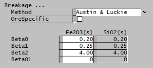
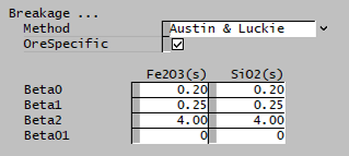
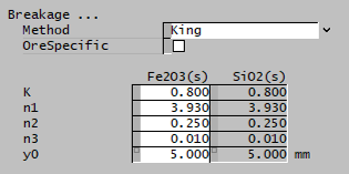
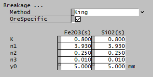
* <math>\text{Breakage method}</math> is the breakage function method, ''0 = User, 1 = Austin & Luckie, 2 = King, 3 = Natural selection'' | |||
* <math>n</math> is the number of size intervals | |||
* <math>m</math> is the number of ore types. | |||
=== Results === | |||
The results are displayed in Excel as an array corresponding to the matrix notation below: | |||
:<math> | |||
\mathit{mdUnit\_HPGR\_Torres} = | |||
\begin{bmatrix} | |||
\begin{bmatrix} | |||
\delta\text{ (t/m}^3\text{)}\\ | |||
x_{\rm c}\text{ (mm)}\\ | |||
\alpha_{\rm IP}\text{ (deg.)}\\ | |||
G_{\rm s}\text{ (t/h)}\\ | |||
U\text{ (m/s)}\\ | |||
\text{Rolls rotational speed (rpm)}\\ | |||
\dot m\text{ (t.s/m}^3\text{.h)}\\ | |||
F\text{ (kN)}\\ | |||
W\text{ (kWh/t)}\\ | |||
P\text{ (kW)}\\ | |||
\end{bmatrix} | |||
& | |||
\begin{array}{c} | |||
\begin{bmatrix} | |||
d_1\text{ (mm)}\\ | |||
\vdots\\ | |||
d_n\text{ (mm)} | |||
\end{bmatrix} | |||
& | |||
\begin{bmatrix} | |||
(Q_{\rm M,P})_{11}\text{ (t/h)} & \dots & (Q_{\rm M,P})_{1m}\text{ (t/h)}\\ | |||
\vdots & \ddots & \vdots\\ | |||
(Q_{\rm M,P})_{n1}\text{ (t/h)} & \dots & (Q_{\rm M,P})_{nm}\text{ (t/h)}\\ | |||
\end{bmatrix} | |||
& | |||
\begin{bmatrix} | |||
(Q_{\rm M,E})_{11}\text{ (t/h)} & \dots & (Q_{\rm M,E})_{1m}\text{ (t/h)}\\ | |||
\vdots & \ddots & \vdots\\ | |||
(Q_{\rm M,E})_{n1}\text{ (t/h)} & \dots & (Q_{\rm M,E})_{nm}\text{ (t/h)}\\ | |||
\end{bmatrix} | |||
& | |||
\begin{bmatrix} | |||
(Q_{\rm M,C})_{11}\text{ (t/h)} & \dots & (Q_{\rm M,C})_{1m}\text{ (t/h)}\\ | |||
\vdots & \ddots & \vdots\\ | |||
(Q_{\rm M,C})_{n1}\text{ (t/h)} & \dots & (Q_{\rm M,C})_{nm}\text{ (t/h)}\\ | |||
\end{bmatrix} | |||
& | |||
\begin{bmatrix} | |||
\bar{d}_1\text{ (mm)}\\ | |||
\vdots\\ | |||
\bar{d}_{n}\text{ (mm)}\\ | |||
\end{bmatrix} | |||
& | |||
\begin{bmatrix} | |||
\begin{bmatrix} | |||
S^{\rm E}_1\\ | |||
\vdots\\ | |||
S^{\rm E}_n\\ | |||
\end{bmatrix}_1 | |||
\dots | |||
\begin{bmatrix} | |||
S^{\rm E}_1\\ | |||
\vdots\\ | |||
S^{\rm E}_n\\ | |||
\end{bmatrix}_m | |||
\end{bmatrix} | |||
& | |||
\begin{bmatrix} | |||
\begin{bmatrix} | |||
B_{1,2}\\ | |||
\vdots\\ | |||
B_{n,2}\\ | |||
\end{bmatrix}_1 | |||
\dots | |||
\begin{bmatrix} | |||
B_{1,2}\\ | |||
\vdots\\ | |||
B_{n,2}\\ | |||
\end{bmatrix}_m | |||
\end{bmatrix} | |||
& | |||
\begin{bmatrix} | |||
y_1\text{ (m)}\\ | |||
\vdots\\ | |||
y_{N_{\rm B}}\text{ (m)}\\ | |||
\end{bmatrix} | |||
& | |||
\begin{bmatrix} | |||
P_1\text{ (kW)}\\ | |||
\vdots\\ | |||
P_{N_{\rm B}}\text{ (kW)}\\ | |||
\end{bmatrix} | |||
\\ | |||
\\ | |||
\\ | |||
\\ | |||
\\ | |||
\\ | |||
\\ | |||
\\ | |||
\end{array} | |||
\end{bmatrix} | |||
</math> | |||
where: | |||
* <math>\text{Rolls rotational speed}</math> is the rotational speed of the rolls (rpm) | |||
* <math>Q_{\rm M,P}</math> is the mass flow rate of particles in the overall, combined product (t/h), equivalent to <math>p_i^{\rm HPGR}</math> in Torres and Casali's nomenclature | |||
* <math>Q_{\rm M,E}</math> is the mass flow rate of particles in the ''edge'' product (t/h), equivalent to <math>p_i^{\rm E}</math> in Torres and Casali's nomenclature | |||
* <math>Q_{\rm M,C}</math> is the mass flow rate of particles in the ''centre'' product (t/h), equivalent to <math>p_i^{\rm C}</math> in Torres and Casali's nomenclature | |||
* <math>B_{ij}</math> is the cumulative breakage function, i.e. <math>b_{ij} = B_{ij} - B_{i+1,j}</math>. | |||
=== Example === | |||
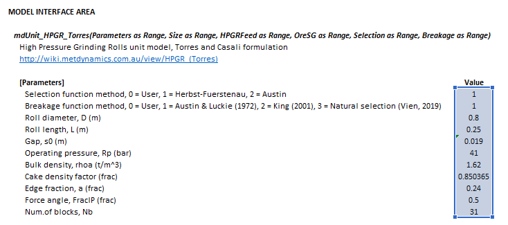
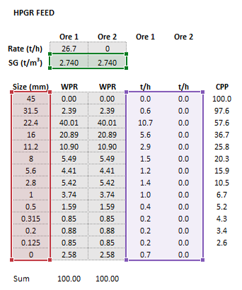
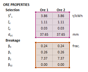
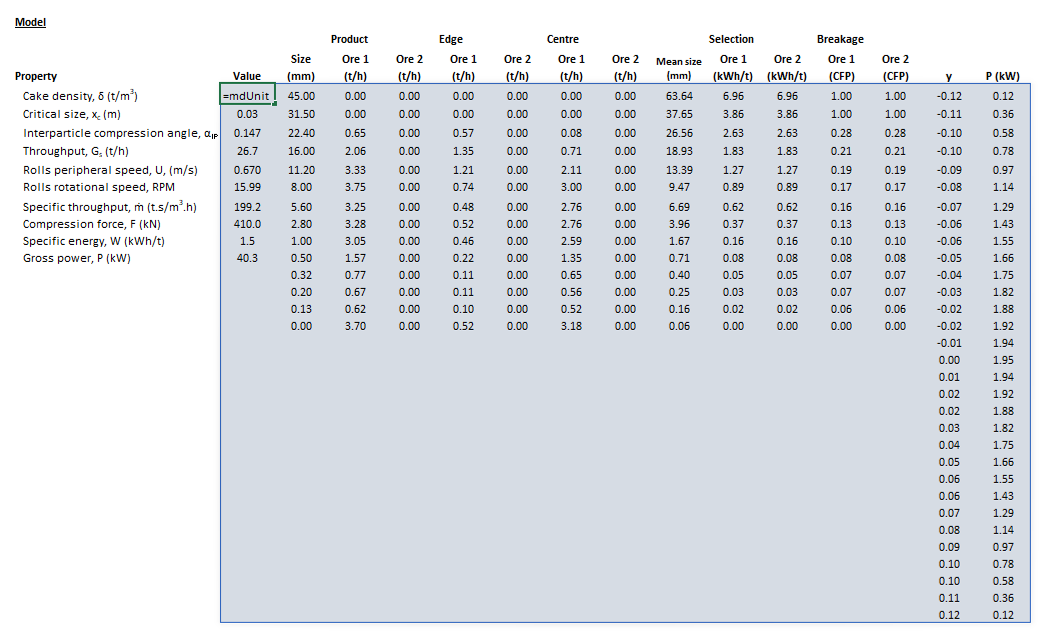
The images below show the selection of input arrays and output results in the Excel interface. | |||
{| | |||
|- style="vertical-align:top;" | |||
| [[File:HPGRTorres1.png|left|frame|Figure 5. Example showing the selection of the '''Parameters''' (blue frame) array in Excel.]]|| [[File:HPGRTorres2.png|left|frame|Figure 6. Example showing the selection of the '''Size''' (red frame), '''HPGRFeed''' (purple frame) and '''OreSG''' (green frame) arrays in Excel.]] || [[File:HPGRTorres3.png|left|frame|Figure 7. Example showing the selection of the '''Selection''' (pink frame) and '''Breakage''' (brown frame) arrays in Excel.]] | |||
|- | |||
|colspan="3"| [[File:HPGRTorres4.png|left|frame|Figure 8. Example showing the outline of the '''Results''' (light blue frame) array in Excel.]] | |||
|} | |||
== SysCAD == | == SysCAD == | ||
{{ | The sections and variable names used in the SysCAD interface are described in detail in the following tables. | ||
{{SysCAD (Page, HPGR, DLL*HPGR)}} | |||
{{SysCAD (Page, HPGR, Torres, HPGR)|Method=Torres}} | |||
{{SysCAD (Page, Mill, Herbst-Fuerstenau, Selection)}} | |||
{{SysCAD (Page, Mill, Herbst-Fuerstenau, Breakage)}} | |||
{{SysCAD (Page, HPGR, Torres, Power)}} | |||
{{SysCAD (Page, About)}} | |||
==== Additional notes ==== | |||
{{SysCAD (Text, HPGR, No PSD Splits)}} | |||
== See also == | |||
* [[HPGR (Morrell-Tondo-Shi)|Morrell-Tondo-Shi HPGR model]] | |||
* [[HPGR (Campos)|Campos HPGR model]] | |||
* [[Mill (Herbst-Fuerstenau)| Herbst-Fuerstenau mill model]] | |||
== External links == | |||
* [https://help.syscad.net/Met_Dynamics_-_HPGR Met Dynamics - HPGR (help.syscad.net)] | |||
* [https://help.syscad.net/Example_-_09_Met_Dynamics_Projects#Crushing_and_Grinding_Example Crushing and Grinding Example project (help.syscad.net)] | |||
* [https://help.syscad.net/Example_-_09_Met_Dynamics_Projects#Crushing,_Grinding_and_Flotation_Example Crushing, Grinding and Flotation Example project (help.syscad.net)] | |||
== References == | == References == | ||
Latest revision as of 13:27, 1 May 2025
Description
This article describes the Torres and Casali (2009) model for comminution by High Pressure Grinding Rolls (HPGR).[1]
Model theory
Throughput
Power
Single particle compression
Interparticle compression
Power distribution profile
Size reduction
Selection and breakage functions
HPGR products
Specific throughput
Excel
The Torres HPGR model may be invoked from the Excel formula bar with the following function call:
=mdUnit_HPGR_Torres(Parameters as Range, Size as Range, HPGRFeed as Range, OreSG as Range, Selection as Range, Breakage as Range)
Invoking the function with no arguments will print Help text associated with the model, including a link to this page.
Inputs
The required inputs are defined below in matrix notation with elements corresponding to cells in Excel row ([math]\displaystyle{ i }[/math]) x column ([math]\displaystyle{ j }[/math]) format:
- [math]\displaystyle{ Parameters= \begin{bmatrix} \text{ Selection function method}\\ \text{ Breakage function method}\\ D\text{ (m)}\\ L\text{ (m)}\\ s_0\text{ (m)}\\ R_{\rm p}\text{ (bar)}\\ \rho_{\rm a}\text{ (t/m}^3\text{)}\\ C_{\rho}\text{ (frac)}\\ a\text{ (frac)}\\ C_{\rm IP}\text{ (frac)}\\ N_{\rm B} \end{bmatrix},\;\;\;\;\;\; Size = \begin{bmatrix} d_{1}\text{ (mm)}\\ \vdots\\ d_n\text{ (mm)}\\ \end{bmatrix},\;\;\;\;\;\; \mathit{HPGRFeed}= \begin{bmatrix} (Q_{\rm M,F})_{11}\text{ (t/h)} & \dots & (Q_{\rm M,F})_{1m}\text{ (t/h)}\\ \vdots & \ddots & \vdots\\ (Q_{\rm M,F})_{n1}\text{ (t/h)} & \dots & (Q_{\rm M,F})_{nm}\text{ (t/h)}\\ \end{bmatrix},\;\;\;\;\;\; OreSG= \begin{bmatrix} (\rho_{\rm S})_{1}\text{ (t/m}^\text{3}\text{)} & \dots & (\rho_{\rm S})_m\text{ (t/m}^\text{3}\text{)}\\ \end{bmatrix} }[/math]
- [math]\displaystyle{ Selection = \begin{cases} \begin{bmatrix} \begin{bmatrix} S^{\rm E}_{1}\\ \vdots\\ S^{\rm E}_{n}\\ \end{bmatrix}_1 \dots \begin{bmatrix} S^{\rm E}_{1}\\ \vdots\\ S^{\rm E}_{n}\\ \end{bmatrix}_m \end{bmatrix} & \text{ Selection function method}=0\text{ (User defined)}\\ & &\\ \begin{bmatrix} \begin{bmatrix} S^{\rm E}_{1}\\ \zeta_1\\ \zeta_2\\ d_{{\rm p}1}\text{ (mm)}\\ \end{bmatrix}_1 \dots \begin{bmatrix} S^{\rm E}_{1}\\ \zeta_1\\ \zeta_2\\ d_{{\rm p}1}\text{ (mm)}\\ \end{bmatrix}_m \end{bmatrix} & \text{ Selection function method}=1\text{ (Herbst-Fuerstenau)}\\ & &\\ \begin{bmatrix} \begin{bmatrix} \alpha_0\\ \alpha_1\\ \alpha_2\\ d_{\rm crit}\text{ (mm)}\\ \alpha_{02}\\ \alpha_{12}\\ \end{bmatrix}_1 \dots \begin{bmatrix} \alpha_0\\ \alpha_1\\ \alpha_2\\ d_{\rm crit}\text{ (mm)}\\ \alpha_{02}\\ \alpha_{12}\\ \end{bmatrix}_m \end{bmatrix} & \text{ Selection function method}=2\text{ (Austin)}\\ \end{cases} }[/math]
- [math]\displaystyle{ Breakage = \begin{cases} \begin{bmatrix} \begin{bmatrix} b_{11} & & 0\\ \vdots & \ddots & \\ b_{n1} & \dots & b_{nn}\\ \end{bmatrix}_1\\ \vdots\\ \begin{bmatrix} b_{11} & & 0\\ \vdots & \ddots & \\ b_{n1} & \dots & b_{nn}\\ \end{bmatrix}_m\\ \end{bmatrix} & \text{ Breakage function method}=0\text{ (User defined)}\\ & &\\ \begin{bmatrix} \begin{bmatrix} \beta_0\\ \beta_1\\ \beta_2\\ \beta_{02}\\ \end{bmatrix}_1 \dots \begin{bmatrix} \beta_0\\ \beta_1\\ \beta_2\\ \beta_{02}\\ \end{bmatrix}_m \end{bmatrix} & \text{ Breakage function method}=1\text{ (Austin and Luckie)}\\ & &\\ \begin{bmatrix} \begin{bmatrix} K\\ n_1\\ n_2\\ n_3\\ y_0\text{ (mm)}\\ \end{bmatrix}_1 \dots \begin{bmatrix} K\\ n_1\\ n_2\\ n_3\\ y_0\text{ (mm)}\\ \end{bmatrix}_m \end{bmatrix} & \text{ Breakage function method}=2\text{ (King)}\\ & &\\ \bigg [ \;\;\; \bigg ] & \text{ Breakage function method}=3\text{ (Natural selection)}\\ \end{cases} }[/math]
where:
- [math]\displaystyle{ \text{Selection method} }[/math] is the selection function method, 0 = User, 1 = Herbst-Fuerstenau, 2 = Austin
- [math]\displaystyle{ \text{Breakage method} }[/math] is the breakage function method, 0 = User, 1 = Austin & Luckie, 2 = King, 3 = Natural selection
- [math]\displaystyle{ n }[/math] is the number of size intervals
- [math]\displaystyle{ m }[/math] is the number of ore types.
Results
The results are displayed in Excel as an array corresponding to the matrix notation below:
- [math]\displaystyle{ \mathit{mdUnit\_HPGR\_Torres} = \begin{bmatrix} \begin{bmatrix} \delta\text{ (t/m}^3\text{)}\\ x_{\rm c}\text{ (mm)}\\ \alpha_{\rm IP}\text{ (deg.)}\\ G_{\rm s}\text{ (t/h)}\\ U\text{ (m/s)}\\ \text{Rolls rotational speed (rpm)}\\ \dot m\text{ (t.s/m}^3\text{.h)}\\ F\text{ (kN)}\\ W\text{ (kWh/t)}\\ P\text{ (kW)}\\ \end{bmatrix} & \begin{array}{c} \begin{bmatrix} d_1\text{ (mm)}\\ \vdots\\ d_n\text{ (mm)} \end{bmatrix} & \begin{bmatrix} (Q_{\rm M,P})_{11}\text{ (t/h)} & \dots & (Q_{\rm M,P})_{1m}\text{ (t/h)}\\ \vdots & \ddots & \vdots\\ (Q_{\rm M,P})_{n1}\text{ (t/h)} & \dots & (Q_{\rm M,P})_{nm}\text{ (t/h)}\\ \end{bmatrix} & \begin{bmatrix} (Q_{\rm M,E})_{11}\text{ (t/h)} & \dots & (Q_{\rm M,E})_{1m}\text{ (t/h)}\\ \vdots & \ddots & \vdots\\ (Q_{\rm M,E})_{n1}\text{ (t/h)} & \dots & (Q_{\rm M,E})_{nm}\text{ (t/h)}\\ \end{bmatrix} & \begin{bmatrix} (Q_{\rm M,C})_{11}\text{ (t/h)} & \dots & (Q_{\rm M,C})_{1m}\text{ (t/h)}\\ \vdots & \ddots & \vdots\\ (Q_{\rm M,C})_{n1}\text{ (t/h)} & \dots & (Q_{\rm M,C})_{nm}\text{ (t/h)}\\ \end{bmatrix} & \begin{bmatrix} \bar{d}_1\text{ (mm)}\\ \vdots\\ \bar{d}_{n}\text{ (mm)}\\ \end{bmatrix} & \begin{bmatrix} \begin{bmatrix} S^{\rm E}_1\\ \vdots\\ S^{\rm E}_n\\ \end{bmatrix}_1 \dots \begin{bmatrix} S^{\rm E}_1\\ \vdots\\ S^{\rm E}_n\\ \end{bmatrix}_m \end{bmatrix} & \begin{bmatrix} \begin{bmatrix} B_{1,2}\\ \vdots\\ B_{n,2}\\ \end{bmatrix}_1 \dots \begin{bmatrix} B_{1,2}\\ \vdots\\ B_{n,2}\\ \end{bmatrix}_m \end{bmatrix} & \begin{bmatrix} y_1\text{ (m)}\\ \vdots\\ y_{N_{\rm B}}\text{ (m)}\\ \end{bmatrix} & \begin{bmatrix} P_1\text{ (kW)}\\ \vdots\\ P_{N_{\rm B}}\text{ (kW)}\\ \end{bmatrix} \\ \\ \\ \\ \\ \\ \\ \\ \end{array} \end{bmatrix} }[/math]
where:
- [math]\displaystyle{ \text{Rolls rotational speed} }[/math] is the rotational speed of the rolls (rpm)
- [math]\displaystyle{ Q_{\rm M,P} }[/math] is the mass flow rate of particles in the overall, combined product (t/h), equivalent to [math]\displaystyle{ p_i^{\rm HPGR} }[/math] in Torres and Casali's nomenclature
- [math]\displaystyle{ Q_{\rm M,E} }[/math] is the mass flow rate of particles in the edge product (t/h), equivalent to [math]\displaystyle{ p_i^{\rm E} }[/math] in Torres and Casali's nomenclature
- [math]\displaystyle{ Q_{\rm M,C} }[/math] is the mass flow rate of particles in the centre product (t/h), equivalent to [math]\displaystyle{ p_i^{\rm C} }[/math] in Torres and Casali's nomenclature
- [math]\displaystyle{ B_{ij} }[/math] is the cumulative breakage function, i.e. [math]\displaystyle{ b_{ij} = B_{ij} - B_{i+1,j} }[/math].
Example
The images below show the selection of input arrays and output results in the Excel interface.
SysCAD
The sections and variable names used in the SysCAD interface are described in detail in the following tables.
MD_HPGR page
The first tab page in the access window will have this name.
| Tag (Long/Short) | Input / Display | Description/Calculated Variables/Options |
|---|---|---|
| Tag | Display | This name tag may be modified with the change tag option. |
| Condition | Display | OK if no errors/warnings, otherwise lists errors/warnings. |
| ConditionCount | Display | The current number of errors/warnings. If condition is OK, returns 0. |
| GeneralDescription / GenDesc | Display | This is an automatically generated description for the unit. If the user has entered text in the 'EqpDesc' field on the Info tab (see below), this will be displayed here.
If this field is blank, then SysCAD will display the unit class ID. |
| Requirements | ||
| On | CheckBox | This enables the unit. If this box is not checked, then the material will pass straight through the crusher with no change to the size distribution. |
| NumParallelUnits | Input | The number of parallel, identical units to simulate:
|
| Method | Fixed Discharge | The discharge particle size distribution is user defined. Different distributions can be used for different solids. |
| Morrell-Shi-Tondo | The throughput, power draw and product size distribution are determined by the Morrell-Tondo-Shi model. Different parameters can be used for different solids. | |
| Torres | The throughput, power draw and product size distribution are determined by the Torres model. Different parameters can be used for different solids. | |
| Campos | The throughput, power draw and product size distribution are determined by the Campos model. Different parameters can be used for different solids. | |
| Options | ||
| ShowQFeed | CheckBox | QFeed and associated tab pages (eg Sp) will become visible, showing the properties of the combined feed stream. |
| ShowQProd | CheckBox | QProd and associated tab pages (eg Sp) will become visible, showing the properties of the products. |
| SizeForPassingFracCalc | Input | Size fraction for % Passing calculation. The size fraction input here will be shown in the Stream Summary section. |
| FracForPassingSizeCalc | Input | Fraction passing for Size calculation. The fraction input here will be shown in the Stream Summary section. |
| Stream Summary | ||
| MassFlow / Qm | Display | The total mass flow in each stream. |
| SolidMassFlow / SQm | Display | The Solids mass flow in each stream. |
| LiquidMassFlow / LQm | Display | The Liquid mass flow in each stream. |
| VolFlow / Qv | Display | The total Volume flow in each stream. |
| Temperature / T | Display | The Temperature of each stream. |
| Density / Rho | Display | The Density of each stream. |
| SolidFrac / Sf | Display | The Solid Fraction in each stream. |
| LiquidFrac / Lf | Display | The Liquid Fraction in each stream. |
| Passing | Display | The mass fraction passing the user-specified size (in the field SizeForPassingFracCalc) in each stream. |
| Passes | Display | The user-specified (in the field FracForPassesSizeCalc) fraction of material in each stream will pass this size fraction. |
HPGR page
The HPGR page is used to specify the input parameters for the HPGR model.
| Tag (Long/Short) | Input / Display | Description/Calculated Variables/Options |
|---|---|---|
| Torres | ||
| HelpLink | Opens a link to this page using the system default web browser. Note: Internet access is required. | |
| Parameters | ||
| RollDiameter / D | Input | Diameter of the rolls. |
| RollLength / L | Input | Length of the rolls. |
| Gap / s0 | Input | Gap between the rolls. |
| OperatingPressure / Rp | Input | Operating pressure of the rolls. |
| FeedBulkDensity / Rhoa | Input | Bulk density of solids in the feed. |
| CakeDensityFactor | Input | Cake density factor. |
| EdgeFraction / a | Input | Fraction of the product collected from the edge of the rolls length, appearing in the edge product stream. |
| ForceAngleFactor | Input | Factor applied to alphaIP when computing power draw. |
| NumBlocks / Nb | Input | Number of model blocks, i.e. instances of the Herbst-Fuerstenau mill model along the length of the rolls. |
| Selection | ||
| Method | User | The user specifies the selection function. |
| Herbst and Fuerstenau | The Herbst and Fuerstenau selection function is used. | |
| Austin | The Austin selection function is used. | |
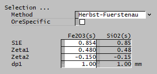
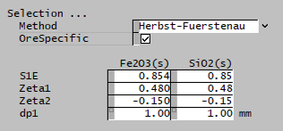
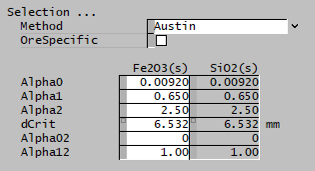
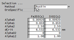
| OreSpecific | CheckBox | Ore-specific parameters, allows the selection function to be separately input for all species. Default is all species have the same set of single input properties. This option is only available if there is more than one species in the project with the size distribution property. |
| The fields below are only visible if Herbst-Fuerstenau is selected. | ||
| S1E | Input | Input parameter of the Herbst-Fuerstenau selection function. |
| Zeta1 | Input | Input parameter of the Herbst-Fuerstenau selection function. |
| Zeta2 | Input | Input parameter of the Herbst-Fuerstenau selection function. |
| dp1 | Input | Input parameter of the Herbst-Fuerstenau selection function. |
| The fields below are only visible if Austin is selected. | ||
| Alpha0 | Input | Input parameter of the Austin selection function. |
| Alpha1 | Input | Input parameter of the Austin selection function. |
| Alpha2 | Input | Input parameter of the Austin selection function. |
| dCrit | Input | Input parameter of the Austin selection function. |
| Alpha02 | Input | Input parameter of the Austin selection function. |
| Alpha12 | Input | Input parameter of the Austin selection function. |
| Breakage | ||
| Method | User | The user specifies the breakage function. |
| Austin and Luckie | The Austin and Luckie breakage function is used. | |
| King | The King selection function is used. | |
| Natural Selection | The Natural selection function is used. | |
| OreSpecific | CheckBox | Ore-specific parameters, allows the breakage function to be separately input for all species. Default is all species have the same set of single input properties. This option is only available if there is more than one species in the project with the size distribution property. |
| The fields below are only visible if Austin and Luckie is selected. | ||
| Beta0 | Input | Input parameter of the Austin and Luckie breakage function. |
| Beta1 | Input | Input parameter of the Austin and Luckie breakage function. |
| Beta2 | Input | Input parameter of the Austin and Luckie breakage function. |
| Beta01 | Input | Input parameter of the Austin and Luckie breakage function. |
| The fields below are only visible if King is selected. | ||
| K | Input | Input parameter of the King breakage function. |
| n1 | Input | Input parameter of the King breakage function. |
| n2 | Input | Input parameter of the King breakage function. |
| n3 | Input | Input parameter of the King breakage function. |
| y0 | Input | Input parameter of the King breakage function. |
| Results | ||
| CakeDensity / delta | Display | Solids density of the cake. |
| CriticalSize / xc | Display | Critical size. |
| InterparComprAngle / alphaIP | Display | Interparticle compression angle. |
| Throughput / Gs | Display | Solids mass throughput flow rate of the HPGR. |
| RollsVelocity / U | Display | Circumferential velocity of the rolls. |
| RollsSpeed | Display | Rotational speed of the rolls. |
| SpecificThroughput / mDot | Display | Specific throughput parameter of the HPGR unit. |
| CompressionForce / F | Display | Compression force of the rolls. |
| GrossPower / P | Display | Gross power draw of the HPGR unit |
| SpecificEnergy / W | Display | Specific energy of grinding. |
Selection page
The Selection page is used to specify or display the selection function values.
| Tag (Long/Short) | Input / Display | Description/Calculated Variables/Options |
|---|---|---|
| Distribution | ||
| Name | Display | Shows the name of the SysCAD Size Distribution (PSD) quality associated with the feed stream. |
| IntervalCount | Display | Shows the number of size intervals in the SysCAD Size Distribution (PSD) quality associated with the feed stream. |
| SpWithPSDCount | Display | Shows the number of species in the feed stream assigned with the SysCAD Size Distribution (PSD) quality. |
| Selection | ||
| Size | Display | Size of each interval in mesh series. |
| MeanSize | Display | Geometric mean size of each interval in mesh series. |
| Selection | Input/Display | Value of the selection function for each size interval, for each ore species. |
Breakage page
The Breakage page is used to specify or display the breakage function values.
| Tag (Long/Short) | Input / Display | Description/Calculated Variables/Options |
|---|---|---|
| Distribution | ||
| Name | Display | Shows the name of the SysCAD Size Distribution (PSD) quality associated with the feed stream. |
| IntervalCount | Display | Shows the number of size intervals in the SysCAD Size Distribution (PSD) quality associated with the feed stream. |
| SpWithPSDCount | Display | Shows the number of species in the feed stream assigned with the SysCAD Size Distribution (PSD) quality. |
| Breakage | ||
| Size | Display | Size of each interval in internal mesh series. |
| Breakage | Input/Display | Value of the breakage function for each parent size interval, progeny size interval and ore species. |
Power page
The Power page is used to display power draw of model blocks along the length of the rolls.
| Tag (Long/Short) | Input / Display | Description/Calculated Variables/Options |
|---|---|---|
| Power | ||
| Position / y | Display | Position along the rolls length. |
| Power / Pk | Display | Power draw of model block at position along the rolls length. |
About page
This page is provides product and licensing information about the Met Dynamics Models SysCAD Add-On.
| Tag (Long/Short) | Input / Display | Description/Calculated Variables/Options |
|---|---|---|
| About | ||
| HelpLink | Opens a link to the Installation and Licensing page using the system default web browser. Note: Internet access is required. | |
| Information | Copies Product and License information to the Windows clipboard. | |
| Product | ||
| Name | Display | Met Dynamics software product name |
| Version | Display | Met Dynamics software product version number. |
| BuildDate | Display | Build date and time of the Met Dynamics Models SysCAD Add-On. |
| License | ||
| File | This is used to locate a Met Dynamics software license file. | |
| Location | Display | Type of Met Dynamics software license or file name and path of license file. |
| SiteCode | Display | Unique machine identifier for license authorisation. |
| ReqdAuth | Display | Authorisation level required, MD-SysCAD Full or MD-SysCAD Runtime. |
| Status | Display | License status, LICENSE_OK indicates a valid license, other messages report licensing errors. |
| IssuedTo | Display | Only visible if Met Dynamics license file is used. Name of organisation/seat the license is authorised to. |
| ExpiryDate | Display | Only visible if Met Dynamics license file is used. License expiry date. |
| DaysLeft | Display | Only visible if Met Dynamics license file is used. Days left before the license expires. |
Additional notes
When the edge stream is connected, the following applies to mass splits:
- Solid species without a particle size distribution property are split to the edge stream according to the overall mass split of the default particle size distribution species selected in the SysCAD Project Configuration
- If the default particle size distribution species is not present in the unit feed, the overall split of all other species with particle size distributions combined is used, as determined by the model.
- Liquids species are split between the edge and product streams in the same proportion as solid species.
- Gas phase species report directly to the product stream without split.
See also
External links
- Met Dynamics - HPGR (help.syscad.net)
- Crushing and Grinding Example project (help.syscad.net)
- Crushing, Grinding and Flotation Example project (help.syscad.net)
References
- ↑ Torres, M. and Casali, A., 2009. A novel approach for the modelling of high-pressure grinding rolls. Minerals Engineering, 22(13), pp.1137-1146.
