Distributions: Difference between revisions
imported>Scott.Munro m (→Swebrec) |
imported>Scott.Munro m (→Model theory) |
||
| (One intermediate revision by the same user not shown) | |||
| Line 4: | Line 4: | ||
== Model theory == | == Model theory == | ||
{{Restricted content}} | |||
<hide> | |||
[[File:Distributions4.png|thumb|450px|Figure 1. Example particle size distributions, log-linear axes.]] | |||
[[File:Distributions5.png|thumb|450px|Figure 2. Example particle size distributions, log-log axes.]] | |||
=== Gaudin-Schuhmann === | === Gaudin-Schuhmann === | ||
| Line 53: | Line 60: | ||
where <math>a</math> is a proportion parameter and <math>c</math> is an undulation exponent. | where <math>a</math> is a proportion parameter and <math>c</math> is an undulation exponent. | ||
</hide> | |||
== Excel == | == Excel == | ||
| Line 101: | Line 109: | ||
|} | |} | ||
| | | | ||
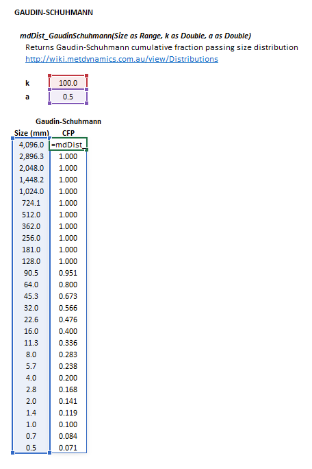
::[[File:Distributions1.png|frame|Figure | ::[[File:Distributions1.png|frame|Figure 3. Example showing the selection of the '''Size''' (blue frame), '''k''' (red frame), '''a''' (purple frame) and '''Results''' (light blue frame) arrays in Excel.]] | ||
|} | |} | ||
| Line 151: | Line 159: | ||
|} | |} | ||
| | | | ||
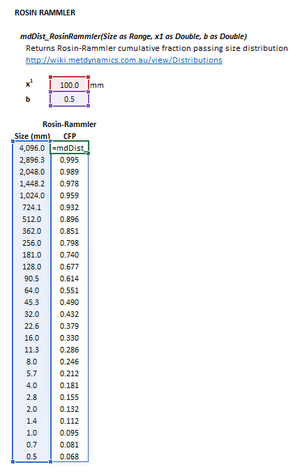
::[[File:Distributions2.png|frame|Figure | ::[[File:Distributions2.png|frame|Figure 4. Example showing the selection of the '''Size''' (blue frame), '''x1''' (red frame), '''b''' (purple frame) and '''Results''' (light blue frame) arrays in Excel.]] | ||
|} | |} | ||
| Line 207: | Line 215: | ||
|} | |} | ||
| | | | ||
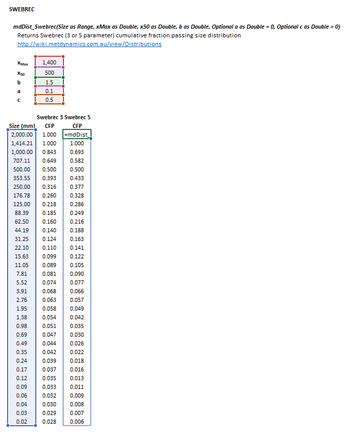
::[[File:Distributions3.png|frame|Figure | ::[[File:Distributions3.png|frame|Figure 5. Example showing the selection of the '''Size''' (blue frame), '''xMax''' (red frame), '''x50''' (purple frame), '''b''' (green frame),'''a''' (pink frame), '''c''' (brown frame) and '''Results''' (light blue frame) arrays in Excel.]] | ||
|} | |} | ||
Latest revision as of 11:32, 4 December 2024
Description
This article describes methods for estimating particle size distributions using the Gaudin-Schuhmann, Rosin-Rammler and Swebrec equations.[1][2]
Model theory
Excel
Gaudin-Schuhmann
The Gaudin-Schuhmann distribution may be invoked from the Excel formula bar with the following function calls:
=mdDist_GaudinSchuhmann(Size as Range, k as Double, m as Double)
Invoking the function with no arguments will print Help text associated with the model, including a link to this page.
The input parameters and calculation results are defined below in matrix notation, along with an example image showing the selection of the same cells and arrays in the Excel interface:
|
| ||||
Rosin-Rammler
The Rosin-Rammler distribution may be invoked from the Excel formula bar with the following function calls:
=mdDist_RosinRammler(Size as Range, x1 as Double, b as Double)
Invoking the function with no arguments will print Help text associated with the model, including a link to this page.
The input parameters and calculation results are defined below in matrix notation, along with an example image showing the selection of the same cells and arrays in the Excel interface:
|
| ||||
Swebrec
The Swebrec distribution may be invoked from the Excel formula bar with the following function calls:
=mdDist_Swebrec(Size as Range, xMax as Double, x50 as Double, b as Double, Optional a as Double = 1, Optional c as Double = 0)
Invoking the function with no arguments will print Help text associated with the model, including a link to this page.
The input parameters and calculation results are defined below in matrix notation, along with an example image showing the selection of the same cells and arrays in the Excel interface:
|
| ||||
![{\displaystyle {\begin{aligned}{\mathit {Size}}&={\begin{bmatrix}d_{1}{\text{ (mm)}}\\\vdots \\d_{n}{\text{ (mm)}}\\\end{bmatrix}}\\\\{\mathit {k}}&={\big [}k{\text{ (mm)}}{\big ]}\\\\{\mathit {a}}&={\big [}a{\big ]}\end{aligned}}}](https://wikimedia.org/api/rest_v1/media/math/render/svg/4156f5409a76c00992afc57bfe79d9641382cfcc)


![{\displaystyle {\begin{aligned}{\mathit {Size}}&={\begin{bmatrix}d_{1}{\text{ (mm)}}\\\vdots \\d_{n}{\text{ (mm)}}\\\end{bmatrix}}\\\\{\mathit {x1}}&={\big [}x^{1}{\text{ (mm)}}{\big ]}\\\\{\mathit {b}}&={\big [}b{\big ]}\end{aligned}}}](https://wikimedia.org/api/rest_v1/media/math/render/svg/7a8dd83daa2de3e8713704a23bb15f1002f1e766)


![{\displaystyle {\begin{aligned}{\mathit {Size}}&={\begin{bmatrix}d_{1}{\text{ (mm)}}\\\vdots \\d_{n}{\text{ (mm)}}\\\end{bmatrix}}\\\\{\mathit {xMax}}&={\big [}x_{\rm {Max}}{\text{ (mm)}}{\big ]}\\\\{\mathit {x50}}&={\big [}x_{50}{\text{ (mm)}}{\big ]}\\\\{\mathit {b}}&={\big [}b{\big ]}\\\\{\mathit {a}}&={\big [}a{\big ]}^{*}\\\\{\mathit {c}}&={\big [}c{\big ]}^{*}\end{aligned}}}](https://wikimedia.org/api/rest_v1/media/math/render/svg/0e671f8c9f28b143dae17921c879fc61f703d52e)


