Blasting (KCO)

Description

This article describes the Kuznetsov–Cunningham–Ouchterlony (KCO) model (Ouchterlony, 2005) for predicting rock fragmentation by blasting.

Model theory

Swebrec distribution

Figure 1. Schematic of blast design geometry (after Bergman, 2005).

The KCO model links blasting conditions to the particle size distribution of fragmented rock via the three-parameter Swebrec function:

$P_{i}={\dfrac {1}{1+\left[{\dfrac {\ln \left({\dfrac {x_{\rm {max}}}{d_{i}}}\right)}{\ln \left({\dfrac {x_{\rm {max}}}{x_{50}}}\right)}}\right]^{b}}}$

where:

• $i$ is the index of the size interval, $i=\{1,2,\dots ,p\}$, $p$ is the number of size intervals
• $P_{i}$ is the cumulative fraction passing size interval $i$
• $d_{i}$ is the size of the square mesh interval that mass is retained on (mm)
• $d_{i+1}<d_{i}<d_{i-1}$, i.e. descending size order from top size ($d_{1}$) to sub mesh ($d_{p}=0$ mm)
• $x_{\rm {max}}$ is the maximum (top) size of the distribution, i.e. the maximum block size (mm)
• $x_{50}$ is the mean size (passing 50%) of the distribution (mm)
• $b$ is a curve-undulation exponent.

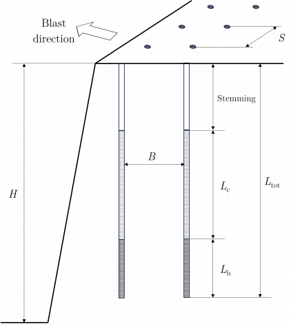
Figure 1 outlines the primary blast design dimensions relevant to the KCO model.

Maximum block size, x_max

The maximum block size is the smallest value of the in situ block size, the blast-hole burden, $B$, and the spacing, $S$, (m), i.e.:

$x_{\rm {max}}=\min\{{\textit {in}}{\text{ }}{\textit {situ}}{\text{ block size}},S,B\}$

Mean size parameter, x₅₀

The mean size of the distribution, $x_{50}$ (mm), is estimated by:

$x_{50}={\dfrac {g(n)\cdot A\cdot Q^{\frac {1}{6}}\cdot \left({\dfrac {115}{s_{\rm {ANFO}}}}\right)^{\frac {19}{30}}}{q^{0.8}}}\cdot 10$

where:

• $A$ is the rock mass factor
• $Q$ is the charge weight per hole (kg)
• $s_{\rm {ANFO}}$ is the explosive’s weight strength relative to ANFO (%)
• $q$ is the specific charge (kg/m³)
• $g(n)=1$ is assumed
• The 10 factor converts Ouchterlony's centimetre units to millimetres.

The rock mass factor, $A$ is:

$A=0.06({\mathit {RMD}}+{\mathit {RDI}}+{\mathit {HF}})$

The rock mass description,${\mathit {RMD}}$, is:

${\mathit {RMD}}={\begin{cases}10&{\text{Powdery/friable}}\\{\mathit {JF}}&{\text{Vertical joints}}\\50&{\text{Massive}}\\\end{cases}}$

The joint factor, ${\mathit {JF}}$,

${\mathit {JF}}={\mathit {JPS}}+{\mathit {JPA}}$

where the joint plane spacing, ${\mathit {JF}}$, is related to the aversge joint spacing, $S_{\rm {J}}$ (m), by:

${\mathit {JPS}}={\begin{cases}10&S_{\rm {J}}<0.1{\text{ m}}\\20&0.1{\text{ m}}<S_{\rm {J}}\leq {\text{oversize }}x_{\rm {o}}\\50&S_{\rm {J}}>{\text{oversize }}x_{\rm {o}}\\\end{cases}}$

The joint plane angle, ${\mathit {JPA}}$, is:

${\mathit {JPA}}={\begin{cases}20&{\text{Dip out of face}}\\30&{\text{Strike perpendicular to face}}\\40&{\text{Dip into face}}\\\end{cases}}$

The rock density influence, ${\mathit {RDI}}$, is:

${\mathit {RDI}}=0.025\rho -50$

where $\rho$ is the rock density (kg/m³).

The hardness factor, ${\mathit {HF}}$, is:

${\mathit {HF}}={\begin{cases}{\dfrac {E}{3}}&E<50\\{\dfrac {\sigma _{\rm {c}}}{5}}&E\geq 50\\\end{cases}}$

where $E$ is Young's Modulus (GPa) and $\sigma _{\rm {c}}$ is the compressive strength of the rock (MPa).

Curve-undulation exponent, b

The curve-undulation exponent $b$ is determined from:

$b=\left[2\ln 2\cdot \ln \left({\dfrac {x_{\rm {max}}}{x_{50}}}\right)\right]\cdot n$

where:

$n=\left(2.2-{\dfrac {0.014B}{\varnothing _{\rm {h}}}}\right)\cdot \left(1-{\dfrac {\mathit {SD}}{B}}\right)\cdot {\sqrt {\dfrac {\left(1+{\dfrac {S}{B}}\right)}{2}}}\cdot \left[{\dfrac {\left\vert L_{\rm {b}}-L_{\rm {c}}\right\vert }{L_{\rm {tot}}}}+1\right]^{0.1}\cdot \left({\dfrac {L_{\rm {tot}}}{H}}\right)$

and:

• $\varnothing _{\rm {h}}$ is the drill-hole diameter (m)
• $L_{\rm {b}}$ is the length of bottom charge (m)
• $L_{\rm {c}}$ is the length of column charge (m)
• $L_{\rm {tot}}$ is the total charge length (m)
• $H$ is the bench height or hole depth (m)
• ${\mathit {SD}}$ is the standard deviation of drilling accuracy (m).

Excel

The KCO blasting model may be invoked from the Excel formula bar with the following function call:

=mdUnit_Blasting_KCO(Parameters as Range, Size as Range)

Invoking the function with no arguments will print Help text associated with the model, including a link to this page.

Inputs

The required inputs are defined below in matrix notation with elements corresponding to cells in Excel row ($i$) x column ($j$) format:

$Parameters={\begin{bmatrix}H{\text{ (m)}}\\B{\text{ (m)}}\\S{\text{ (m)}}\\\varnothing _{\rm {h}}{\text{ (m)}}\\L_{\rm {b}}{\text{ (m)}}\\L_{\rm {c}}{\text{ (m)}}\\L_{\rm {Tot}}{\text{ (m)}}\\{\mathit {SD}}{\text{ (m)}}\\Q{\text{ (kg)}}\\q{\text{ (kg/m}}^{3}{\text{)}}\\s_{\rm {ANFO}}{\text{ (}}\%{\text{)}}\\\rho {\text{ (t/m}}^{3}{\text{)}}\\\sigma _{\rm {c}}{\text{ (MPa)}}\\E{\text{ (GPa)}}\\{\textit {In}}{\text{ }}{\textit {situ}}{\text{ block size (m)}}\\{\mathit {RMD}}\\\end{bmatrix}},\;\;\;\;\;\;Size={\begin{bmatrix}d_{1}{\text{ (mm)}}\\\vdots \\d_{p}{\text{ (mm)}}\\\end{bmatrix}}$

Results

The results are displayed in Excel as an array corresponding to the matrix notation below:

${\mathit {mdUnit\_Blasting\_KCO}}={\begin{bmatrix}{\begin{bmatrix}{\mathit {RMD}}\\{\mathit {RDI}}\\{\mathit {HF}}\\x_{\rm {max}}{\text{ (mm)}}\\n\\g(n)\\x_{50}{\text{ (mm)}}\\b\\\end{bmatrix}}&{\begin{array}{c}{\begin{bmatrix}{\mathit {P}}_{1}{\text{ (w/w)}}\\\vdots \\{\mathit {P}}_{p}{\text{ (w/w)}}\end{bmatrix}}\\\\\\\\\end{array}}\end{bmatrix}}$

Example

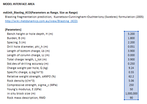
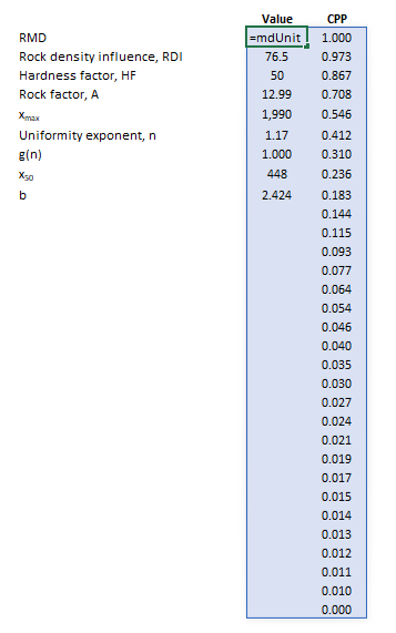
The images below show the selection of input arrays and output results in the Excel interface.

Figure 1. Example showing the selection of the Parameters (blue frame) array in Excel.

Figure 2. Example showing the selection of the Size (red frame) array in Excel.

Figure 3. Example showing the selection of the Results (light blue frame) array in Excel.

See also

• Distributions (Swebrec)