Distributions: Difference between revisions
md>Scott.Munro m (→Description) |
imported>Scott.Munro m (→Excel) |
||
| (2 intermediate revisions by 2 users not shown) | |||
| Line 5: | Line 5: | ||
== Model theory == | == Model theory == | ||
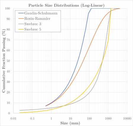
{{ | [[File:Distributions4.png|thumb|450px|Figure 1. Example particle size distributions, log-linear axes.]] | ||
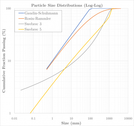
[[File:Distributions5.png|thumb|450px|Figure 2. Example particle size distributions, log-log axes.]] | |||
=== Gaudin-Schuhmann === | |||
The Gaudin-Schuhmann distribution is:{{Gupta and Yan (2016)}} | |||
:<math>P_i = \left ( \dfrac{d_i}{k} \right )^a</math> | |||
where: | |||
* <math>i</math> is the index of the size interval, <math>i = \{1,2,\dots,n\}</math>, <math>n</math> is the number of size intervals | |||
* <math>P_i</math> is the cumulative fraction passing size interval <math>i</math> | |||
* <math>d_i</math> is the size of the square mesh interval that mass is retained on (mm) | |||
* <math>d_{i+1}<d_i<d_{i-1}</math>, i.e. descending size order from top size (<math>d_{1}</math>) to sub mesh (<math>d_{n}=0</math> mm) | |||
* <math>k</math> the Gaudin-Schuhmann size parameter (mm) | |||
* <math>a</math> the Gaudin-Schuhmann distribution parameter | |||
=== Rosin-Rammler === | |||
The Rosin-Rammler distribution is:{{Gupta and Yan (2016)}} | |||
:<math>P_i = \exp \left [ - \left ( \dfrac{d_i}{x^1} \right )^b \right ]</math> | |||
where: | |||
* <math>i</math> is the index of the size interval, <math>i = \{1,2,\dots,n\}</math>, <math>n</math> is the number of size intervals | |||
* <math>P_i</math> is the cumulative fraction passing size interval <math>i</math> | |||
* <math>d_i</math> is the size of the square mesh interval that mass is retained on (mm) | |||
* <math>d_{i+1}<d_i<d_{i-1}</math>, i.e. descending size order from top size (<math>d_{1}</math>) to sub mesh (<math>d_{n}=0</math> mm) | |||
* <math>x^1</math> is the Rosin-Rammler size parameter (mm) | |||
* <math>b</math> is the Rosin-Rammler distribution parameter | |||
=== Swebrec === | |||
The basic three-parameter Swebrec function is:{{Ouchterlony (2005)}} | |||
:<math>P_i = \dfrac{1}{1 + \left [ \dfrac{\ln \left ( \dfrac{x_{\rm max}}{d_i} \right )}{\ln \left ( \dfrac{x_{\rm max}}{x_{50}} \right )} \right ]^b }</math> | |||
where: | |||
* <math>i</math> is the index of the size interval, <math>i = \{1,2,\dots,n\}</math>, <math>n</math> is the number of size intervals | |||
* <math>P_i</math> is the cumulative fraction passing size interval <math>i</math> | |||
* <math>d_i</math> is the size of the square mesh interval that mass is retained on (mm) | |||
* <math>d_{i+1}<d_i<d_{i-1}</math>, i.e. descending size order from top size (<math>d_{1}</math>) to sub mesh (<math>d_{n}=0</math> mm) | |||
* <math>x_{\rm Max}</math> is the maximum (top) size of the distribution (mm) | |||
* <math>x_{50}</math> is the mean size (passing 50%) of the distribution (mm) | |||
* <math>b</math> is a curve-undulation exponent | |||
The extended five-parameter Swebrec function is: | |||
:<math>P_i = \dfrac{1}{1 + a \left [ \dfrac{\ln \left ( \dfrac{x_{\rm max}}{d_i} \right )}{\ln \left ( \dfrac{x_{\rm max}}{x_{50}} \right )} \right ]^b + (1 - a) \left [ \dfrac{ \left ( \dfrac{x_{\rm max}}{d_i} - 1 \right )}{ \left ( \dfrac{x_{\rm max}}{x_{50}} - 1 \right )} \right ]^c}</math> | |||
where <math>a</math> is a proportion parameter and <math>c</math> is an undulation exponent. | |||
== Excel == | == Excel == | ||
| Line 51: | Line 102: | ||
|- style="vertical-align:top;" | |- style="vertical-align:top;" | ||
|colspan="2"| | |colspan="2"| | ||
|} | |} | ||
| | | | ||
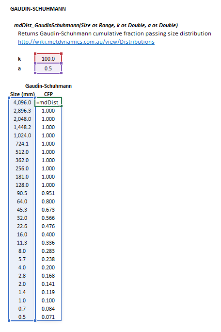
::[[File:Distributions1.png|frame|Figure | ::[[File:Distributions1.png|frame|Figure 3. Example showing the selection of the '''Size''' (blue frame), '''k''' (red frame), '''a''' (purple frame) and '''Results''' (light blue frame) arrays in Excel.]] | ||
|} | |} | ||
| Line 107: | Line 153: | ||
* <math>d_i</math> is the size of the square mesh interval that feed mass is retained on (mm) | * <math>d_i</math> is the size of the square mesh interval that feed mass is retained on (mm) | ||
* <math>d_{i+1}<d_i<d_{i-1}</math>, i.e. descending size order from top size (<math>d_{1}</math>) to sub mesh (<math>d_{n}=0</math> mm) | * <math>d_{i+1}<d_i<d_{i-1}</math>, i.e. descending size order from top size (<math>d_{1}</math>) to sub mesh (<math>d_{n}=0</math> mm) | ||
|} | |} | ||
| | | | ||
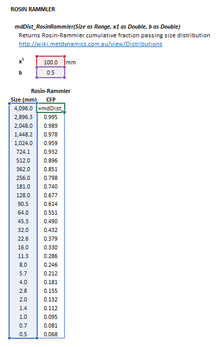
::[[File:Distributions2.png|frame|Figure | ::[[File:Distributions2.png|frame|Figure 4. Example showing the selection of the '''Size''' (blue frame), '''x1''' (red frame), '''b''' (purple frame) and '''Results''' (light blue frame) arrays in Excel.]] | ||
|} | |} | ||
| Line 119: | Line 162: | ||
The Swebrec distribution may be invoked from the Excel formula bar with the following function calls: | The Swebrec distribution may be invoked from the Excel formula bar with the following function calls: | ||
<syntaxhighlight lang="vb">=mdDist_Swebrec(Size as Range, xMax as Double, x50 as Double, b as Double, Optional a as Double = | <syntaxhighlight lang="vb">=mdDist_Swebrec(Size as Range, xMax as Double, x50 as Double, b as Double, Optional a as Double = 1, Optional c as Double = 0)</syntaxhighlight> | ||
{{Excel (Text, Help, No Arguments)}} | {{Excel (Text, Help, No Arguments)}} | ||
| Line 146: | Line 189: | ||
\mathit{b} & = \big [ b \big ]\\ | \mathit{b} & = \big [ b \big ]\\ | ||
\\ | \\ | ||
\mathit{a} & = \big [ a \big ]\\ | \mathit{a} & = \big [ a \big ]^*\\ | ||
\\ | \\ | ||
\mathit{c} & = \big [ c \big ] | \mathit{c} & = \big [ c \big ]^* | ||
\end{align}</math> | \end{align}</math> | ||
| | | | ||
| Line 163: | Line 206: | ||
|- style="vertical-align:top;" | |- style="vertical-align:top;" | ||
|colspan="2"| | |colspan="2"| | ||
where | where <math>^*</math> represents optional parameters. | ||
* | Omitting both optional parameters will invoke the three-parameter Swebrec function, otherwise the five-parameter version is used. | ||
|} | |} | ||
| | | | ||
::[[File:Distributions3.png|frame|Figure | ::[[File:Distributions3.png|frame|Figure 5. Example showing the selection of the '''Size''' (blue frame), '''xMax''' (red frame), '''x50''' (purple frame), '''b''' (green frame),'''a''' (pink frame), '''c''' (brown frame) and '''Results''' (light blue frame) arrays in Excel.]] | ||
|} | |} | ||
Latest revision as of 13:26, 29 January 2024
Description
This article describes methods for estimating particle size distributions using the Gaudin-Schuhmann, Rosin-Rammler and Swebrec equations.[1][2]
Model theory
Gaudin-Schuhmann
The Gaudin-Schuhmann distribution is:[1]
where:
- is the index of the size interval, , is the number of size intervals
- is the cumulative fraction passing size interval
- is the size of the square mesh interval that mass is retained on (mm)
- , i.e. descending size order from top size () to sub mesh ( mm)
- the Gaudin-Schuhmann size parameter (mm)
- the Gaudin-Schuhmann distribution parameter
Rosin-Rammler
The Rosin-Rammler distribution is:[1]
where:
- is the index of the size interval, , is the number of size intervals
- is the cumulative fraction passing size interval
- is the size of the square mesh interval that mass is retained on (mm)
- , i.e. descending size order from top size () to sub mesh ( mm)
- is the Rosin-Rammler size parameter (mm)
- is the Rosin-Rammler distribution parameter
Swebrec
The basic three-parameter Swebrec function is:[2]
where:
- is the index of the size interval, , is the number of size intervals
- is the cumulative fraction passing size interval
- is the size of the square mesh interval that mass is retained on (mm)
- , i.e. descending size order from top size () to sub mesh ( mm)
- is the maximum (top) size of the distribution (mm)
- is the mean size (passing 50%) of the distribution (mm)
- is a curve-undulation exponent
The extended five-parameter Swebrec function is:
where is a proportion parameter and is an undulation exponent.
Excel
Gaudin-Schuhmann
The Gaudin-Schuhmann distribution may be invoked from the Excel formula bar with the following function calls:
=mdDist_GaudinSchuhmann(Size as Range, k as Double, m as Double)
Invoking the function with no arguments will print Help text associated with the model, including a link to this page.
The input parameters and calculation results are defined below in matrix notation, along with an example image showing the selection of the same cells and arrays in the Excel interface:
|
| ||||
Rosin-Rammler
The Rosin-Rammler distribution may be invoked from the Excel formula bar with the following function calls:
=mdDist_RosinRammler(Size as Range, x1 as Double, b as Double)
Invoking the function with no arguments will print Help text associated with the model, including a link to this page.
The input parameters and calculation results are defined below in matrix notation, along with an example image showing the selection of the same cells and arrays in the Excel interface:
|
| ||||
Swebrec
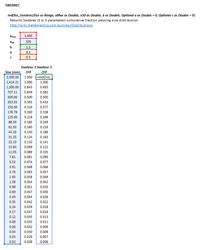
The Swebrec distribution may be invoked from the Excel formula bar with the following function calls:
=mdDist_Swebrec(Size as Range, xMax as Double, x50 as Double, b as Double, Optional a as Double = 1, Optional c as Double = 0)
Invoking the function with no arguments will print Help text associated with the model, including a link to this page.
The input parameters and calculation results are defined below in matrix notation, along with an example image showing the selection of the same cells and arrays in the Excel interface:
|
| ||||


![{\displaystyle P_{i}=\exp \left[-\left({\dfrac {d_{i}}{x^{1}}}\right)^{b}\right]}](https://wikimedia.org/api/rest_v1/media/math/render/svg/a91a39653b0fb5db0443f08b9d4e8bebc1365887)


![{\displaystyle P_{i}={\dfrac {1}{1+\left[{\dfrac {\ln \left({\dfrac {x_{\rm {max}}}{d_{i}}}\right)}{\ln \left({\dfrac {x_{\rm {max}}}{x_{50}}}\right)}}\right]^{b}}}}](https://wikimedia.org/api/rest_v1/media/math/render/svg/a710659c0e1d32749f21ed00284b5ae0e059cf19)


![{\displaystyle P_{i}={\dfrac {1}{1+a\left[{\dfrac {\ln \left({\dfrac {x_{\rm {max}}}{d_{i}}}\right)}{\ln \left({\dfrac {x_{\rm {max}}}{x_{50}}}\right)}}\right]^{b}+(1-a)\left[{\dfrac {\left({\dfrac {x_{\rm {max}}}{d_{i}}}-1\right)}{\left({\dfrac {x_{\rm {max}}}{x_{50}}}-1\right)}}\right]^{c}}}}](https://wikimedia.org/api/rest_v1/media/math/render/svg/3e9b5e55199a2780cf8f546624fe7227cdf34628)

![{\displaystyle {\begin{aligned}{\mathit {Size}}&={\begin{bmatrix}d_{1}{\text{ (mm)}}\\\vdots \\d_{n}{\text{ (mm)}}\\\end{bmatrix}}\\\\{\mathit {k}}&={\big [}k{\text{ (mm)}}{\big ]}\\\\{\mathit {a}}&={\big [}a{\big ]}\end{aligned}}}](https://wikimedia.org/api/rest_v1/media/math/render/svg/4156f5409a76c00992afc57bfe79d9641382cfcc)

![{\displaystyle {\begin{aligned}{\mathit {Size}}&={\begin{bmatrix}d_{1}{\text{ (mm)}}\\\vdots \\d_{n}{\text{ (mm)}}\\\end{bmatrix}}\\\\{\mathit {x1}}&={\big [}x^{1}{\text{ (mm)}}{\big ]}\\\\{\mathit {b}}&={\big [}b{\big ]}\end{aligned}}}](https://wikimedia.org/api/rest_v1/media/math/render/svg/7a8dd83daa2de3e8713704a23bb15f1002f1e766)

![{\displaystyle {\begin{aligned}{\mathit {Size}}&={\begin{bmatrix}d_{1}{\text{ (mm)}}\\\vdots \\d_{n}{\text{ (mm)}}\\\end{bmatrix}}\\\\{\mathit {xMax}}&={\big [}x_{\rm {Max}}{\text{ (mm)}}{\big ]}\\\\{\mathit {x50}}&={\big [}x_{50}{\text{ (mm)}}{\big ]}\\\\{\mathit {b}}&={\big [}b{\big ]}\\\\{\mathit {a}}&={\big [}a{\big ]}^{*}\\\\{\mathit {c}}&={\big [}c{\big ]}^{*}\end{aligned}}}](https://wikimedia.org/api/rest_v1/media/math/render/svg/0e671f8c9f28b143dae17921c879fc61f703d52e)


