Interpolation

Description

This article describes linear and cubic spline data interpolation methods.

Model theory

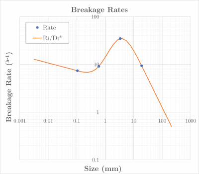
Figure 1. An example of cubic spline interpolation with linear extrapolation at the extents.

Linear interpolation

Linear interpolation is a technique for approximating the value of a function between two known data points. It involves constructing a straight line that passes through the two given points and using this line to estimate the value of the function at an intermediate point.

Given two data points $(x_{1},y_{1})$ and $(x_{2},y_{2})$, where $x_{1}<x_{2}$, the linear interpolation formula to estimate the value $y$ at a point $x$ within the interval $(x_{1},x_{2})$ is:

$y=y_{1}+{\frac {x-x_{1}}{x_{2}-x_{1}}}(y_{2}-y_{1})$

Linear interpolation provides a simple and computationally efficient method for approximating function values.

Cubic spline interpolation

Cubic spline interpolation uses a piecewise cubic polynomial to approximate a function smoothly between known data points.

Given a set of distinct data points $(x_{1},y_{1}),(x_{2},y_{2}),\dots ,(x_{n},y_{n})$, where $x_{1}<x_{2}<\dots <x_{n}$, a cubic spline interpolator constructs a piecewise cubic polynomial $S(x)$ that satisfies the following conditions:

1. Interpolation: $S(x_{i})=y_{i}$ for $i=1,2,\dots ,n$. (The spline passes through all data points.)
2. Smoothness: $S(x)$ and its first two derivatives are continuous across the entire interval $[x_{1},x_{n}]$. (The spline has no abrupt changes in its slope or curvature.)

Cubic splines offer enhanced accuracy and flexibility compared to linear interpolation, especially for functions with nonlinear behavior.

This implementation of cubic spines also applies linear extrapolation at the extents of the data set, as illustrated in Figure 1.

Please see the Wikipedia article on Spline interpolation or references such as Napier-Munn et al. (1996) for a more detailed description of cubic spline interpolation.

Excel

The interpolation methods may be invoked from the Excel formula bar with the following function calls:

=mdInterp_Linear(known_xs as Range, known_ys as Range, xs as Range)

and

=mdInterp_CubicSpline(known_xs as Range, known_ys as Range, xs as Range)

Invoking the function with no arguments will print Help text associated with the model, including a link to this page.

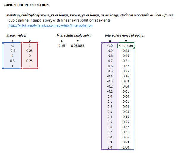
The input parameters and calculation results are defined below in matrix notation, along with an example image showing the selection of the same cells and arrays in the Excel interface:

${\begin{aligned}{\mathit {known\_xs}}={\begin{bmatrix}x_{1}\\\vdots \\x_{n}\\\end{bmatrix}},\;\;\;\;{\mathit {known\_ys}}={\begin{bmatrix}y_{1}\\\vdots \\y_{n}\\\end{bmatrix}},\;\;\;\;{\mathit {xs}}={\begin{bmatrix}x_{1}\\\vdots \\x_{m}\\\end{bmatrix}}\;\;\;\;\end{aligned}}$ ${\begin{aligned}{\mathit {mdInterp\_Linear}}&={\begin{bmatrix}y_{1}\\\vdots \\y_{m}\\\end{bmatrix}}\\\\{\mathit {mdInterp\_CubicSpline}}&={\begin{bmatrix}y_{1}\\\vdots \\y_{m}\\\end{bmatrix}}\end{aligned}}$ where: $n$ is the number of data points $m$ is the number of interpolation points $x_{1}\cdots x_{n}$ is an array of the known independent data values $y_{1}\cdots y_{n}$ is an array of the known dependent data values $x_{1}\cdots x_{m}$ is an array of the independent data values at which the dependant variable is to be interpolated $y_{1}\cdots y_{m}$ is an array of the interpolated dependant variable values

Figure 1. Example showing the selection of the known_xs (blue frame), known_ys (red frame), xs (purple frame), and Results (light blue frame) arrays in Excel.

References

- ↑ Napier-Munn, T.J., Morrell, S., Morrison, R.D. and Kojovic, T., 1996. Mineral comminution circuits: their operation and optimisation. Julius Kruttschnitt Mineral Research Centre, Indooroopilly, QLD.